Introduction

The development of modelling approaches that approximate and describe the data generating processes underlying the observed data in as much detail as possible is a guiding principle in both statistics and machine learning. We therefore strongly agree with the statement of Hothorn et al. (2014) that ''the ultimate goal of any regression analysis is to obtain information about the entire conditional distribution $F_{Y}(y|\mathbf{x})$ of a response given a set of explanatory variables''.

''Practitioners expect forecasting to reduce future uncertainty by providing accurate predictions like those in hard sciences. However, this is a great misconception. A major purpose of forecasting is not to reduce uncertainty but reveal its full extent and implications by estimating it as precisely as possible. [...] The challenge for the forecasting field is how to persuade practitioners of the reality that all forecasts are uncertain and that this uncertainty cannot be ignored, as doing so could lead to catastrophic consequences.'' Makridakis (2022b)

It has not been too long, though, that most regression models focused on estimating the conditional mean $\mathbb{E}(Y|\mathbf{X} = \mathbf{x})$ only, implicitly treating higher moments of the conditional distribution $F_{Y}(y|\mathbf{x})$ as fixed nuisance parameters. As such, models that minimize an $\ell_{2}$-type loss for the conditional mean are not able to fully exploit the information contained in the data, since this is equivalent to assuming a Normal distribution with constant variance. In real world situations, however, the data generating process is usually less well behaved, exhibiting characteristics such as heteroskedasticity, varying degrees of skewness and kurtosis or intermittent and sporadic behaviour. In recent years, however, there has been a clear shift in both academic and corporate research toward modelling the entire conditional distribution. This change in attention is most evident in the recent M5 forecasting competition (Makridakis et al., 2022a,b), which differed from previous ones in that it consisted of two parallel competitions: in addition to providing accurate point forecasts, participants were also asked to forecast nine different quantiles to approximate the distribution of future sales.

Distributional Gradient Boosting Machines

This section introduces the general idea of distributional modelling. For a more thorough introduction, we refer the interested reader to Rigby and Stasinopoulos (2005); Klein et al. (2015a,b); Stasinopoulos et al. (2017).

GAMLSS

Probabilistic forecasts are predictions in the form of a probability distribution, rather than a single point estimate only. In this context, the introduction of Generalized Additive Models for Location Scale and Shape (GAMLSS) by Rigby and Stasinopoulos (2005) has stimulated a lot of research and culminated in a new research branch that focuses on modelling the entire conditional distribution in dependence of covariates.

Univariate Targets

In its original formulation, GAMLSS assume a univariate response $y$ to follow a distribution $\mathcal{D}\bigl(\boldsymbol{\theta}(x)\bigr)$ that depends on up to four parameters, i.e., $y_{i} \stackrel{ind}{\sim} \mathcal{D}\bigl(\boldsymbol{\theta}_{i}(x_{i})\bigr)$ with $\boldsymbol{\theta}_{i}(x_{i}) = \bigl(\mu_{i}(x_{i}), \sigma^{2}_{i}(x_{i}), \nu_{i}(x_{i}), \tau_{i}(x_{i})\bigr), i=1,\ldots, N$, where $\mu_{i}(\cdot)$ and $\sigma^{2}_{i}(\cdot)$ are often location and scale parameters, respectively, while $\nu_{i}(\cdot)$ and $\tau_{i}(\cdot)$ correspond to shape parameters such as skewness and kurtosis. Hence, the framework allows to model not only the mean (or location) but all parameters as functions of explanatory variables. It is important to note that distributional modelling implies that observations are independent, but not necessarily identical realizations $y \stackrel{ind}{\sim} \mathcal{D}\big(\boldsymbol{\theta}(x)\big)$, since all distributional parameters $\boldsymbol{\theta}(x)$ are related to and allowed to change with covariates. In contrast to Generalized Linear (GLM) and Generalized Additive Models (GAM), the assumption of the response distribution belonging to an exponential family is relaxed in GAMLSS and replaced by a more general class of distributions, including highly skewed and/or kurtotic continuous, discrete and mixed discrete, as well as zero-inflated distributions. While the original formulation of GAMLSS in Rigby and Stasinopoulos (2005) suggests that any distribution can be described by location, scale and shape parameters, it is not necessarily true that the observed data distribution can actually be characterized by all of these parameters. Hence, we follow Klein et al. (2015b) and use the term distributional modelling and GAMLSS interchangeably.

From a frequentist point of view, distributional modelling can be formulated as follows

\[\begin{equation} y_{i} \stackrel{ind}{\sim} \mathcal{D} \begin{pmatrix} h_{1}\bigl(\theta_{i1}(x_{i})\bigr) = \eta_{i1} \\ h_{2}\bigl(\theta_{i2}(x_{i})\bigr) = \eta_{i2} \\ \vdots \\ h_{K}\bigl(\theta_{iK}(x_{i})\bigr) = \eta_{iK} \end{pmatrix} \end{equation}\]

for $i = 1, \ldots, N$, where $\mathcal{D}$ denotes a parametric distribution for the response $\textbf{y} = (y_{1}, \ldots, y_{N})^{\prime}$ that depends on $K$ distributional parameters $\theta_{k}$, $k = 1, \ldots, K$, and with $h_{k}(\cdot)$ denoting a known function relating distributional parameters to predictors $\eta_{k}$. In its most generic form, the predictor $\eta_{k}$ is given by

\[\begin{equation} \eta_{k} = f_{k}(\mathbf{x}), \qquad k = 1, \ldots, K \end{equation}\]

Within the original distributional regression framework, the functions $f_{k}(\cdot)$ usually represent a combination of linear and GAM-type predictors, which allows to estimate linear effects or categorical variables, as well as highly non-linear and spatial effects using a Spline-based basis function approach. The predictor specification $\eta_{k}$ is generic enough to use tree-based models as well, which allows us to extend XGBoost to a probabilistic framework.

Mixture Distributions

Mixture densities, or mixture distributions, offer an extension to the notion of traditional univariate distributions by allowing the observed data to be thought of as arising from multiple underlying processes. In its essence, a mixture distribution is a weighted combination of several component distributions, where each component contributes to the overall mixture distribution, with the weights indicating the importance of each component. For instance, if you imagine the observed data distribution having multiple modes, a mixture of Gaussians could be employed to capture each mode with a separate Gaussian distribution.

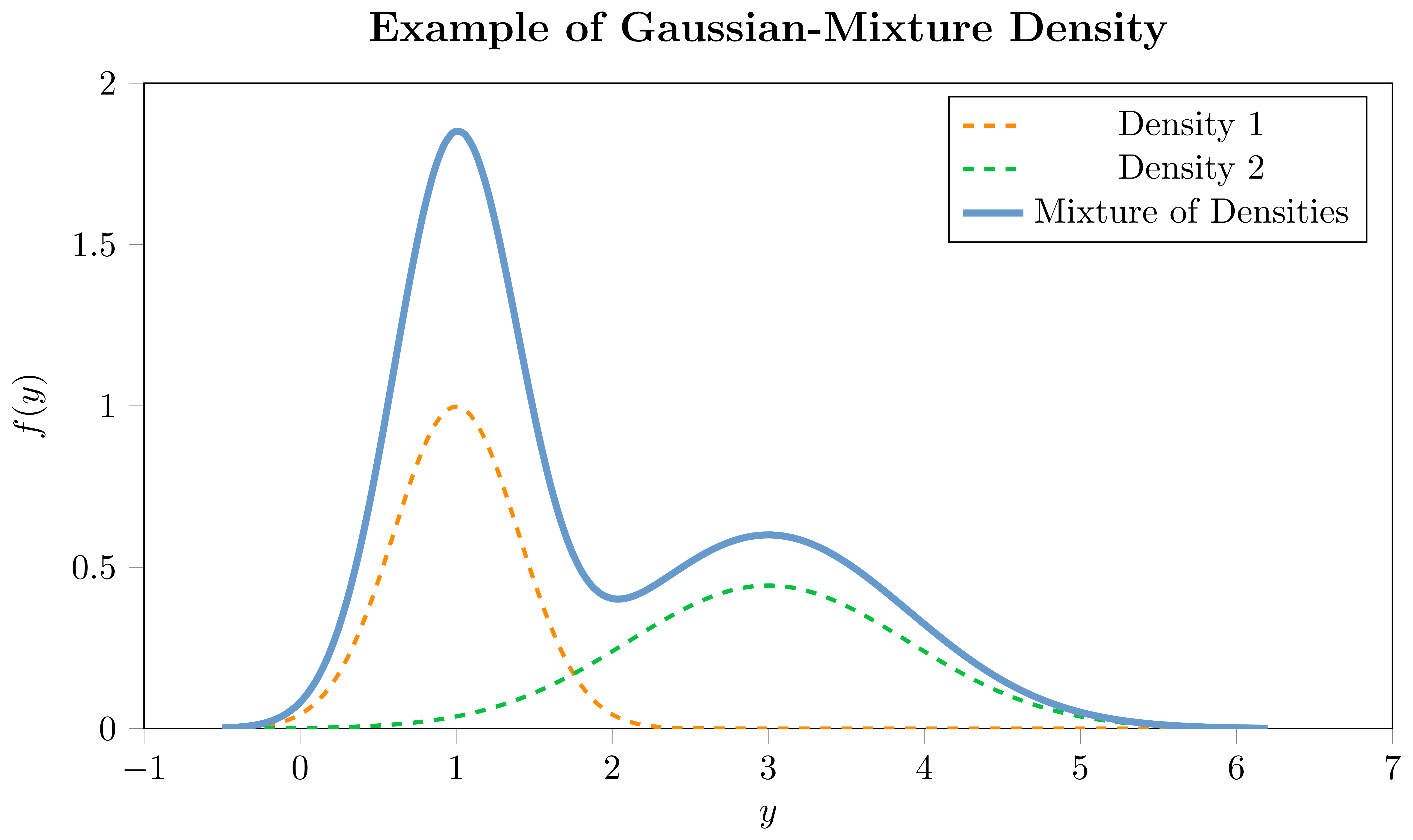
For each component of the mixture, there would be a set of parameters that depend on covariates, and additional mixing coefficients which are also modeled as a function of covariates. This is particularly useful when a single parametric distribution cannot adequately capture the underlying data generating process. A mixture distribution can be represented as follows:

\[\begin{equation} f\bigl(y_{i} | \boldsymbol{\theta}_{i}(x_{i})\bigr) = \sum_{m=1}^{M} w_{i,m}(x_{i}) \cdot f_{m}\bigl(y_{i} | \boldsymbol{\theta}_{i,m}(x_{i})\bigr) \end{equation}\]

where $f(\cdot)$ represents the mixture density for the $i$-th observation, $f_{m}(\cdot)$ is the $m$-th component density, each with its own set of parameters $\boldsymbol{\theta}_{i,m}(\cdot)$, and $w_{i,m}(\cdot)$ represent the weights of the $m$-th component in the mixture, subject to $\sum_{j=1}^{M} w_{i,m} = 1$. The components can either be a combination of different parametric univariate distributions, such as a combination of a Normal and a StudentT, or, as in our implementation, a combination of the same distribution-type with different parameterizations, e.g., Gaussian-Mixture or StudentT-Mixture. The choice of the component distributions depends on the characteristics of the data and the underlying assumptions. Due to their high flexibility, mixture densities can portray a diverse range of shapes, making them adaptable to a plethora of datasets. By incorporating mixture densities within our framework, users can gain a more comprehensive understanding of the conditional distribution of the response variable, providing a more accurate representation of the data generating process. Hence, mixture densities greatly expand the expressive power of distributional modeling frameworks like GAMLSS, allowing one to capture a wider array of data distributions with enhanced flexibility by combining multiple members of this set.

Normalizing Flows

Although the GAMLSS framework offers considerable flexibility, parametric distributions may prove not flexible enough to provide a reasonable approximation for certain dataset, e.g., for multi-modal distributions. For such cases, it is preferable to relax the assumption of a parametric distribution and approximate the data non-parametrically. While there are several alternatives for learning conditional distributions, we propose to use Normalizing Flows for their ability to fit complex distributions with only a few parameters.

The principle that underlies Normalizing Flows is to turn a simple base distribution, e.g., $F_{Z}(\mathbf{z}) = N(0,1)$, into a more complex and realistic distribution of the target variable $F_{Y}(\mathbf{y})$ by applying several bijective transformations $h_{j}$, $j = 1, \ldots, J$ to the variable of the base distribution

\[\begin{equation} \mathbf{y} = h_{J} \circ h_{J-1} \circ \cdots \circ h_{1}(\mathbf{z}) \end{equation}\]

Based on the complete transformation function $h=h_{J}\circ\ldots\circ h_{1}$, the density of $\mathbf{y}$ is then given by the change of variables theorem

\[\begin{equation} f_{Y}(\mathbf{y}) = f_{Z}\big(h(\mathbf{y})\big) \cdot \Bigg|\frac{\partial h(\mathbf{y})}{\partial \mathbf{y}}\Bigg| \end{equation}\]

where scaling with the Jacobian determinant $|h^{\prime}(\mathbf{y})| = |\partial h(\mathbf{y}) / \partial \mathbf{y}|$ ensures $f_{Y}(\mathbf{y})$ to be a proper density integrating to one. The composition of these transformations is invertible, allowing one to sample from the complex distribution by transforming samples from the base distribution.

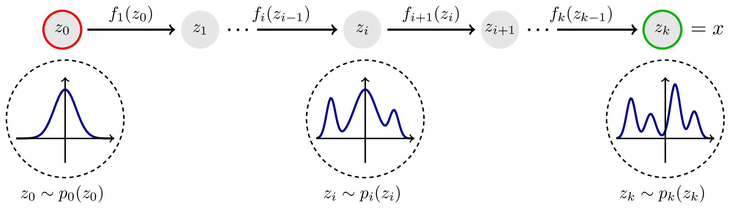
Image source: https://tikz.net/janosh/normalizing-flow.png

Our Normalizing Flow approach is based on element-wise rational splines of linear or quadratic order as introduced by Durkan (2019) and Dolatabadi (2020) and implemented in Pyro, since they offer a combination of functional flexibility and numerical stability. Despite this specific choice, our framework is generic enough to accommodate the use of other parametrizable Normalizing Flows.

Multivariate Targets

To allow for a more flexible framework that explicitly models the dependencies of a $D$-dimensional response $\mathbf{y} = (y_{i1}, \ldots, y_{iD})^{T}, i=1, \ldots, N$, Klein et al. (2015a) introduce a multivariate version of distributional regression. Similar to the univariate case, multivariate distributional regression relates all $\theta_{k}$, $k = 1, \ldots, K$ parameters of a multivariate density $f_{i}\big(y_{i1}, \ldots, y_{iD} | \theta_{i1}(\mathbf{x}\big), \ldots, \theta_{iK}(\mathbf{x})\big)$ to a set of covariates $\mathbf{x}$. A common choice for multivariate probabilistic regression is to assume a multivariate Gaussian distribution, with the density given

\[\begin{equation} f\big(\mathbf{y}|\theta_{\mathbf{x}}\big) = \frac{1}{\sqrt{(2\pi)^{D}|\Sigma_{\mathbf{x}}|}}\exp\left(-\frac{1}{2}(\mathbf{y} - \mu_{\mathbf{x}})^{T} \Sigma^{-1}_{\mathbf{x}} (\mathbf{y} - \mu_{\mathbf{x}})\right) \end{equation}\]

where $\mu_{\mathbf{x}} \in \mathbb{R}^{D}$ represents a vector of conditional means, $\Sigma_{\mathbf{x}}$ is a positive definite symmetric $D \times D$ covariance matrix and $|\cdot|$ denotes the determinant. For the bivariate case $D=2$, $\Sigma_{\mathbf{x}}$ can be expressed as

\[\begin{equation} \Sigma_{i\mathbf{x}} = \begin{bmatrix} \sigma^{2}_{i,1}(\mathbf{x}) & \rho_{i}(\mathbf{x})\sigma_{i,1}(\mathbf{x})\sigma_{i,2}(\mathbf{x}) \\ \rho_{i}(\mathbf{x})\sigma_{i,2}(\mathbf{x})\sigma_{i,1}(\mathbf{x}) & \sigma^{2}_{i,2}(\mathbf{x}) \\ \end{bmatrix} \end{equation}\]

with the variances on the diagonal and the covariances on the off-diagonal, for $ i=1, \ldots, N $. Other examples include the Cholesky Decomposition or a Low-Rank Covariance approximation of the covariance matrix. For additional details and available distributions, see März (2022a).

Gradient Boosting Machines for Location, Scale and Shape

We draw inspiration from GAMLSS and label our model as XGBoost for Location, Scale and Shape (XGBoostLSS). Despite its nominal reference to GAMLSS, our framework is designed in such a way to accommodate the modeling of a wide range of parametrizable distributions that go beyond location, scale and shape. XGBoostLSS requires the specification of a suitable distribution from which Gradients and Hessians are derived. These represent the partial first and second order derivatives of the log-likelihood with respect to the parameter of interest. GBMLSS are based on multi-parameter optimization, where a separate tree is grown for each parameter. Estimation of Gradients and Hessians, as well as the evaluation of the loss function is done simultaneously for all parameters. Gradients and Hessians are derived using PyTorch's automatic differentiation capabilities. The flexibility offered by automatic differentiation allows users to easily implement novel or customized parametric distributions for which Gradients and Hessians are difficult to derive analytically. It also facilitates the usage of Normalizing Flows, or to add additional constraints to the loss function. To improve the convergence and stability of GBMLSS estimation, unconditional Maximum Likelihood estimates of the parameters are used as offset values. To enable a deeper understanding of the data generating process, GBMLSS also provide attribute importance and partial dependence plots using the Shapley-Value approach.

References

C. M. Bishop. Mixture density networks. Technical Report NCRG/4288, Aston University, Birmingham, UK, 1994.
Hadi Mohaghegh Dolatabadi, Sarah Erfani, and Christopher Leckie. Invertible Generative Modeling using Linear Rational Splines. In The 23rd International Conference on Artificial Intelligence and Statistics (AISTATS), 4236–4246, 2020.
Conor Durkan, Artur Bekasov, Iain Murray, and George Papamakarios. Neural Spline Flows. In Proceedings of the 33rd International Conference on Neural Information Processing Systems. 2019.
Nadja Klein, Thomas Kneib, Stephan Klasen, and Stefan Lang. Bayesian structured additive distributional regression for multivariate responses. Journal of the Royal Statistical Society: Series C (Applied Statistics), 64(4):569–591, 2015a.
Nadja Klein, Thomas Kneib, and Stefan Lang. Bayesian Generalized Additive Models for Location, Scale, and Shape for Zero-Inflated and Overdispersed Count Data. Journal of the American Statistical Association, 110(509):405–419, 2015b.
Alexander März. Multi-Target XGBoostLSS Regression. arXiv pre-print, 2022a.
Alexander März, and Thomas Kneib. Distributional Gradient Boosting Machines, 2022b.
Alexander März. XGBoostLSS - An extension of XGBoost to probabilistic forecasting, 2019.
Spyros Makridakis, Evangelos Spiliotis, and Vassilios Assimakopoulos. The M5 competition: Background, organization, and implementation. International Journal of Forecasting, 38(4):1325–1336, 2022a.
Spyros Makridakis, Evangelos Spiliotis, Vassilios Assimakopoulos, Zhi Chen, Anil Gaba, Ilia Tsetlin, and Robert L. Winkler. The M5 uncertainty competition: Results, findings and conclusions. International Journal of Forecasting, 38(4):1365–1385, 2022b.
R. A. Rigby and D. M. Stasinopoulos. Generalized additive models for location, scale and shape. Journal of the Royal Statistical Society: Series C (Applied Statistics), 54(3):507–554, 2005.
Mikis D. Stasinopoulos, Robert A. Rigby, Gillian Z. Heller, Vlasios Voudouris, and Fernanda de Bastiani. Flexible Regression and Smoothing: Using GAMLSS in R. Chapman & Hall / CRC The R Series. CRC Press, London, 2017.