Gradient Boosted Decision Trees (GBDTs) like XGBoost and LightGBM achieve state-of-the-art performance on many tabular datasets. While they partition the feature space and assign constant predictions per region, their leaf values are not simple averages. Instead, GBDTs compute optimal updates using gradient and Hessian information to minimize a loss function via a Newton–Raphson-style procedure.
Modern GBDT implementations such as LightGBM and XGBoost rely on gradients $g_{i}$ and Hessians $h_{i}$, where
\[g_{i} = \frac{\partial \mathcal{L}\bigl(y_{i}, \hat{\psi}_{i}\bigr)}{\partial \hat{\psi}_{i}}, \quad h_{i} = \frac{\partial^{2} \mathcal{L}\bigl(y_{i}, \hat{\psi}_{i}\bigr)}{\partial \hat{\psi}_{i}^2}\]are the first and second order derivatives of a loss function $\mathcal{L}$ with respect to the output $\hat{\psi}_{i}$ for observations $i = 1, \ldots, N$.
Friedman’s (1999) original gradient boosting formulation used only first-order gradients in a technique called gradient descent in function space. Modern implementations like XGBoost (Chen & Guestrin, 2016) and LightGBM (Ke et al., 2017) extended this by incorporating second-order Hessian information, yielding Newton-Raphson-style updates. This second-order approach often leads to faster convergence and better performance.
Think of gradients as directional signals telling us how to reduce the error. If we imagine the loss function as a valley, the gradient points us toward the steepest descent. The Hessian, being the second derivative, tells us about the curvature - how quickly the gradient itself is changing. This curvature information helps us take more intelligent steps, avoiding overshooting the minimum. In the context of GBDTs:
Among others, gradients and Hessians serve two crucial functions in each boosting iteration: they guide the tree construction via split decisions and determine the optimal values assigned to leaf nodes.
During tree building, GBDTs use aggregated gradients and Hessians to make splitting decisions. The algorithm evaluates potential splits by examining how much they would reduce the loss. A greedy approach is used that maximizes the loss reduction:
\[\mathcal{L}_{split} \propto \frac{(\sum_{i\in I_L} g_i)^2}{\sum_{i\in I_L} h_i + \lambda} + \frac{(\sum_{i\in I_R} g_i)^2}{\sum_{i\in I_R} h_i + \lambda} - \frac{(\sum_{i\in I} g_i)^2}{\sum_{i\in I} h_i + \lambda}\]where $I_L$ and $I_R$ denote the instance sets of left and right nodes after a candidate split respectively, and $I = I_L \cup I_R$ represents their union. This is fundamentally different from traditional trees that might split based on variance reduction or Gini impurity.
Once a tree structure is determined, the optimal value for each leaf is calculated using what is essentially a Newton-Raphson step:
\[w^{*}_{j} = - \frac{G_{j}}{H_{j} + \lambda}, \quad \text{with} \quad G_{j} = \sum_{i \in I_{j}} g_{i}, \quad H_{j} = \sum_{i \in I_{j}} h_{i}\]where \(I_{j} = \{i \mid q(x_{i})=j\}\) is the set of indices of observations assigned to the $j$-th leaf, $q(\cdot)$ is the learned tree structure that maps an input to its corresponding leaf $j$, where the leaf assignment is determined by the feature vector $x_i$, and $\lambda$ is a regularization term.
For each leaf, the algorithm computes:
This formula represents a one-step Newton update, not an average. It finds the value that best reduces the loss function given the current gradient and curvature information. Crucially, the loss function determines the outputs from each tree - the leaf values are specifically chosen to minimize the loss function, not to represent simple averages.
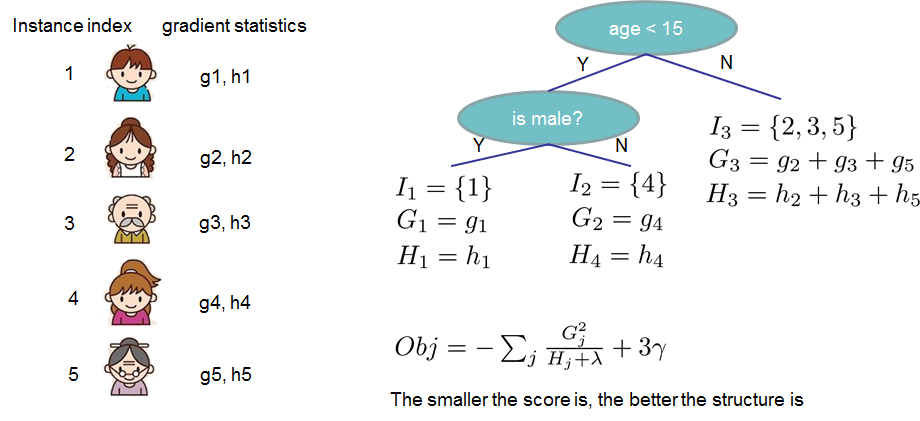
Looking at the illustrated example with five observations being split into a tree:
Source: XGBoost Documentation
When observations are assigned to leaves based on features like age and gender, each observation carries its gradient and Hessian information $(g_1,h_1)$ through $(g_5,h_5)$. The leaf values are not computed by averaging the target values of observations 2, 3, and 5 in leaf 3. Instead, the optimal leaf value is $-G_3/(H_3 + \lambda)$, where $G_3 = g_2 + g_3 + g_5$ and $H_3 = h_2 + h_3 + h_5$.
This aggregation of gradients and Hessians, followed by the Newton-Raphson-style update, allows the tree to make predictions that optimally reduce the loss function - something simple averaging cannot achieve for arbitrary loss functions.
Conventional GBDTs operate in function space, mapping input features $x$ to outputs $\hat{\psi}$ by minimizing a specified loss function. For instance, when using Mean Squared Error (MSE) in a regression setting, $\hat{\psi}$ represents the conditional mean of the target variable. While the use of an $L_{2}$-type loss may suggest that GBDTs create outputs by directly averaging target values, they instead operate through gradient and Hessian-based updates of the following form:
\[\hat{\psi}^{(m)}(x_i) = \hat{\psi}^{(m-1)}(x_i) + \hat{\delta}^{(m)}(x_i), \quad \text{where} \quad \hat{\delta}^{(m)}(x_i) = \eta \cdot w^{*}_{j(i)}\]where:
The leaf weights approximate a Newton-Raphson update, where $w^{*}_{j} = -\frac{G_j}{H_j + \lambda}$ aggregates individual gradients and Hessians across all observations in leaf $j$. This second-order approximation makes GBDTs highly adaptive for a wide range of tasks, allowing $\hat{\psi}$ to represent any quantity as long as the associated loss function is twice-continuously differentiable. Note that while most GBDT objectives assume a twice-differentiable loss, variants exist that use only first-order gradients when Hessians are undefined (e.g., Quantile-Loss).
GBDTs build trees sequentially. At each iteration:
This iterative process, guided entirely by gradients and Hessians rather than target averaging, enables GBDTs to incrementally refine predictions and achieve state-of-the-art performance across diverse machine learning tasks. For the specific case of MSE loss, the gradient is proportional to the residuals, and the Hessian is constant. This can lead to the impression that GBDTs simply fit residuals, when in fact they always follow gradient-based updates derived from the specified loss function. Having understood how gradients and Hessians guide optimization, we can now ask a crucial question: what exactly does this optimization make the model learn? The answer lies in the choice of the loss function.
The choice of loss function fundamentally determines what the GBDT will estimate. This is not merely about how errors are measured - it defines the optimization itself. Through the gradient-based updates described above, GBDTs’ predictions converge toward the function that minimizes the expected loss:
\[f^*(x) = \arg\min_{f} \, \mathbb{E}\big[\mathcal{L}(Y, f(X))\big].\]Different loss functions have different theoretical minimizers, so they lead to estimates of different conditional quantities. In other words, by changing the loss, you change what the model learns.
| Loss Function | Estimated Quantity | Interpretation |
|---|---|---|
| $L_2$ (MSE) | $\mathbb{E}[Y \mid X=x]$ | Conditional mean |
| $L_1$ (MAE) | $\mathrm{median}(Y \mid X=x)$ | Conditional median |
| Quantile loss ($\tau$) | $Q_\tau(Y \mid X=x)$ | Conditional quantile (e.g., 0.1, 0.9) |
| Log-loss | $P(Y=1 \mid X=x)$ | Class probability (for binary classification) |
This explains why GBDT architectures can be adapted to such diverse tasks as regression, quantile estimation, and classification. By merely changing the loss function - and consequently the gradients and Hessians - we redefine what the model’s leaf values represent and what target it approximates.
When using the squared error (MSE or more generally $L_2$ loss), GBDTs are effectively trained to approximate the conditional mean of the target variable given features:
\[f^*(x) = \mathbb{E}[Y|X=x]\]This is a direct consequence of the fact that minimizing $L_2$ risk leads to the conditional expectation as the optimal predictor. Every tree, via gradient and Hessian statistics, is moving the predictions closer to this conditional mean. As explained earlier, the leaf values are computed using a Newton-Raphson step based on aggregated gradients and Hessians, which for $L_2$ loss results in updates that move predictions toward the mean. It is not simple averaging of target values in the leaves that leads to this outcome, but rather the optimization process driven by the loss function.
Assuming that the conditional distribution of the target is Gaussian with constant variance, minimizing MSE is equivalent to performing maximum likelihood estimation under that model. To see why, consider the negative log-likelihood for a normal distribution:
\[-\log p(y|x; \mu, \sigma^2) = \frac{1}{2\sigma^2}(y - \mu(x))^2 + \frac{1}{2}\log(2\pi\sigma^2)\]When we minimize this expression over a dataset with respect to $\mu(x)$, the constant terms do not affect the optimization, leaving us with:
\[\arg\min_{\mu} \sum_{i=1}^{n} \frac{1}{2}(y_i - \mu(x_i))^2\]This is exactly the MSE objective used in LightGBM and XGBoost.
While the $L_2$ loss focuses on the conditional mean, distributional gradient boosting methods such as LightGBMLSS and XGBoostLSS extend the classical GBDT framework from point estimation to full probabilistic modeling. Instead of minimizing a loss with respect to a single target value (mean, median, or quantile), they minimize the negative log-likelihood of a specified probability distribution. This probabilistic extension preserves the same gradient–Hessian optimization mechanism but replaces point-wise losses with distribution-based likelihoods.
This example demonstrates, step by step, how a modern GBDT (e.g., LightGBM/XGBoost) uses gradients and Hessians to choose splits and compute leaf values. It clarifies two common misconceptions: (i) leaf values are not simple averages of targets, and (ii) the model performs gradient-based optimization using the loss function’s derivatives, not residual-fitting (a misleading simplification specific to MSE).
We use five observations with features (price, colour) and sales as the target. We initialize predictions with 0.5 for simplicity.
| id | price | colour | sales $y_i$ |
|---|---|---|---|
| 1 | 8 | red | 5 |
| 2 | 12 | red | 2 |
| 3 | 7 | blue | 6 |
| 4 | 15 | blue | 1 |
| 5 | 9 | red | 4 |
Initial prediction (LightGBM default): \(\hat{\psi}^{(0)} = 0.5 \quad \text{for all observations}\)
Using MSE as implemented in XGBoost/LightGBM:
\[\mathcal{L}(y,\hat{\psi})=\tfrac{1}{2}\,(y-\hat{\psi})^2,\qquad g_i=\frac{\partial \mathcal{L}}{\partial \hat{\psi}_i}=\hat{\psi}_i-y_i,\qquad h_i=\frac{\partial^2 \mathcal{L}}{\partial \hat{\psi}_i^2}=1\]At iteration $m=1$ with $\hat{\psi}^{(0)}=0.5$:
\[g_i=0.5-y_i,\qquad h_i=1\]| id | $g_i$ | $h_i$ |
|---|---|---|
| 1 | $0.5-5=-4.5$ | 1 |
| 2 | $0.5-2=-1.5$ | 1 |
| 3 | $0.5-6=-5.5$ | 1 |
| 4 | $0.5-1=-0.5$ | 1 |
| 5 | $0.5-4=-3.5$ | 1 |
Parent sums: \(\sum_i g_i=(-4.5)+(-1.5)+(-5.5)+(-0.5)+(-3.5)=-15.5,\qquad \sum_i h_i=5\)
The parent term in the split gain is $\frac{(-15.5)^2}{5} = \frac{240.25}{5} = 48.05$.
The split gain used by modern GBDTs is:
\[\text{Gain} = \frac{\big(\sum_{i\in I_L} g_i\big)^2}{\sum_{i\in I_L} h_i + \lambda} + \frac{\big(\sum_{i\in I_R} g_i\big)^2}{\sum_{i\in I_R} h_i + \lambda} - \frac{\big(\sum_{i\in I} g_i\big)^2}{\sum_{i\in I} h_i + \lambda}\]We set $\lambda=0$ for simplicity.
$I_L={1,3,5}$: $G_L=(-4.5)+(-5.5)+(-3.5)=-13.5$, $H_L=3 \Rightarrow \frac{G_L^2}{H_L}=\frac{(-13.5)^2}{3}=\frac{182.25}{3}=60.75$
$I_R={2,4}$: $G_R=(-1.5)+(-0.5)=-2.0$, $H_R=2 \Rightarrow \frac{G_R^2}{H_R}=\frac{(-2.0)^2}{2}=\frac{4.0}{2}=2.0$
$\textbf{Gain}_A = 60.75+2.0-48.05=14.70$
Red $I_{\text{red}}={1,2,5}$: $G_{\text{red}}=(-4.5)+(-1.5)+(-3.5)=-9.5$, $H=3 \Rightarrow \frac{G^2}{H}=\frac{90.25}{3}\approx 30.083$
Blue $I_{\text{blue}}={3,4}$: $G_{\text{blue}}=(-5.5)+(-0.5)=-6.0$, $H=2 \Rightarrow \frac{G^2}{H}=\frac{36.0}{2}=18.0$
$\textbf{Gain}_B = 30.083+18.0-48.05\approx 0.033$
Decision: Choose $\text{price}<10$ since $14.70 \gg 0.033$.
For each leaf $j$:
\[w_j^* = -\frac{G_j}{H_j+\lambda}\]With $\lambda=0$:
Let the learning rate be $\eta=0.3$. The per-sample increment is:
\[\delta^{(1)}(x_i)=\eta\cdot w^*_{j(i)},\qquad \hat{\psi}^{(1)}(x_i)=\hat{\psi}^{(0)}(x_i)+\delta^{(1)}(x_i)\]For the chosen split:
| id | price | colour | leaf | $\delta^{(1)}$ | $\hat{\psi}^{(1)}$ |
|---|---|---|---|---|---|
| 1 | 8 | red | Left | +1.35 | 0.5 + 1.35 = 1.85 |
| 2 | 12 | red | Right | +0.30 | 0.5 + 0.30 = 0.80 |
| 3 | 7 | blue | Left | +1.35 | 1.85 |
| 4 | 15 | blue | Right | +0.30 | 0.80 |
| 5 | 9 | red | Left | +1.35 | 1.85 |
Modern GBDTs use gradient and Hessian information to both construct trees and assign leaf values. The values in leaf nodes are not averages of observations - they are optimization steps designed to reduce the loss function.
Understanding this distinction is crucial. While simple averaging is approximated for squared error loss (and only because the gradient and Hessian lead to this), the mechanism is fundamentally different: GBDTs arrive at predictions through gradient optimization, not simple averaging.
Under $L_2$ loss, any model learns the conditional mean. This ensures strong performance around the center of the target distribution, but systematically over-forecasts the lower tail and under-forecasts the upper tail. For applications where tails matter (risk forecasting, extreme demand spikes, etc.), alternative losses or distributional modeling approaches are necessary.
The flexibility of the gradient boosting framework - its ability to work with any twice differentiable loss function - makes it straightforward to adapt GBDTs to specialized requirements by simply changing the loss function and computing the corresponding gradients and Hessians.
To verify that LightGBM indeed uses the above formulas, we train a simple model and compare the actual leaf weights and predictions of the model to those computed using the above formulas.
import numpy as np
import lightgbm as lgb
from sklearn.datasets import make_regression
from sklearn.model_selection import train_test_split

# Set random seed for reproducibility
seed=123
np.random.seed(seed)

# Generate synthetic regression data
X, y = make_regression(n_samples=1000, n_features=10, noise=10, random_state=seed)
X_train, X_test, y_train, y_test = train_test_split(X, y, test_size=0.2, random_state=seed)
We train a model with:
np.random.seed(seed)

# Define model parameters
params = {
    'objective': 'regression',
    'metric': 'mse',
    'num_leaves': 15,
    'learning_rate': 0.3,
    'lambda_l2': 0.5,
    'verbose': -1,
    'seed': 123,
    'boost_from_average': False,  # Start from 0 as initial prediction
}

# Train model
train_data = lgb.Dataset(X_train, label=y_train)
model = lgb.train(params, train_data, num_boost_round=1)

print(f"Model trained with {params['num_leaves']} leaves")
print(f"Learning rate η = {params['learning_rate']}")
print(f"Regularization λ = {params['lambda_l2']}")
Output:
Model trained with 15 leaves
Learning rate η = 0.3
Regularization λ = 0.5
For the first tree with boost_from_average=False, initial predictions are 0.
For MSE loss:
# Initial predictions are 0
preds_initial = np.zeros(len(X_train))

# Compute gradients and Hessians for MSE
gradients = preds_initial - y_train  # g_i = ŷ_i - y_i = -y_i
hessians = np.ones(len(y_train))     # h_i = 1
# Get leaf assignments for each sample
leaf_indices = model.predict(X_train, num_iteration=1, pred_leaf=True).flatten()

# Extract actual leaf weights from the model
tree_df = model.trees_to_dataframe()
leaf_nodes = tree_df[tree_df['split_gain'].isna()].copy()  # Leaf nodes have no split
leaf_nodes['leaf_num'] = leaf_nodes['node_index'].str.extract(r'L(\d+)').astype(int)
leaf_value_map = dict(zip(leaf_nodes['leaf_num'], leaf_nodes['value']))

print(f"Number of leaves: {len(leaf_value_map)}")
print(f"Unique leaf assignments: {np.unique(leaf_indices)}")
print(f"\nSample of actual leaf weights from LightGBM:")
for leaf_id in sorted(list(leaf_value_map.keys())[:5]):
    print(f"  Leaf {leaf_id}: w = {leaf_value_map[leaf_id]:.6f}")
Output:
Number of leaves: 15
Unique leaf assignments: [ 0  1  2  3  4  5  6  7  8  9 10 11 12 13 14]

Sample of actual leaf weights from LightGBM:
  Leaf 0: w = -89.803428
  Leaf 3: w = -69.701744
  Leaf 5: w = -29.439445
  Leaf 6: w = -16.978203
  Leaf 11: w = -22.564865
Now we compute leaf weights using the formula and compare them to LightGBM’s actual values:
\[w_j^{\text{computed}} = \eta \cdot \left(-\frac{G_j}{H_j + \lambda}\right) = 0.3 \cdot \left(-\frac{\sum_{i \in R_j} g_i}{\sum_{i \in R_j} h_i + 0.5}\right)\]Note: In many implementations, the learning rate $\eta$ is applied during the prediction update step rather than being baked into the leaf weights themselves.
# Extract parameters
eta = params['learning_rate']
lambda_l2 = params['lambda_l2']

# Storage for comparison
actual_weights = []
computed_weights = []
leaf_sizes = []

print(f"Formula: w_j = η · (-Σg_i / (Σh_i + λ))")
print(f"Parameters: η={eta}, λ={lambda_l2}\n")

print("{:<10} {:<15} {:<15} {:<15} {:<12}".format(
    "Leaf", "Actual w_j", "Computed w_j", "Error", "N_samples"))
print("-" * 75)

for leaf_id in sorted(np.unique(leaf_indices)):
    mask = (leaf_indices == leaf_id)
    n_samples = mask.sum()

    # Sum gradients and Hessians in this leaf
    G_j = gradients[mask].sum()
    H_j = hessians[mask].sum()

    # Apply formula
    w_j_computed = eta * (-G_j / (H_j + lambda_l2))
    w_j_actual = leaf_value_map[int(leaf_id)]

    error = abs(w_j_actual - w_j_computed)

    actual_weights.append(w_j_actual)
    computed_weights.append(w_j_computed)
    leaf_sizes.append(n_samples)

    print(f"{leaf_id:<10} {w_j_actual:<15.6f} {w_j_computed:<15.6f} {error:<15.2e} {n_samples:<12}")

actual_weights = np.array(actual_weights)
computed_weights = np.array(computed_weights)
Output:
Formula: w_j = η · (-Σg_i / (Σh_i + λ))
Parameters: η=0.3, λ=0.5

Leaf       Actual w_j      Computed w_j    Error           N_samples
---------------------------------------------------------------------------
0          -89.803428      -89.803429      6.32e-07        62
1          -66.485838      -66.485838      1.81e-07        20
2          -16.484145      -16.484145      3.93e-08        28
3          -69.701744      -69.701743      2.67e-07        28
4          91.781561       91.781561       5.58e-08        68
5          -29.439445      -29.439445      1.42e-07        55
6          -16.978203      -16.978203      1.80e-07        74
7          -5.895929       -5.895929       7.67e-08        49
8          -14.786499      -14.786499      1.92e-07        27
9          37.008983       37.008983       5.94e-08        64
10         45.140052       45.140052       4.16e-08        79
11         -22.564865      -22.564865      1.22e-08        69
12         -13.617065      -13.617065      3.76e-08        56
13         30.433308       30.433308       6.31e-09        76
14         26.782495       26.782495       1.27e-07        45
# Error metrics
mae = np.mean(np.abs(actual_weights - computed_weights))
rmse = np.sqrt(np.mean((actual_weights - computed_weights)**2))
max_error = np.max(np.abs(actual_weights - computed_weights))

print("=" * 80)
print("SUMMARY: Leaf Weights")
print("=" * 80)
print(f"Number of leaves: {len(actual_weights)}")
print(f"Mean Absolute Error between actual and computed weights: {mae:.2e}")
print(f"Root Mean Squared Error between actual and computed weights: {rmse:.2e}")
print(f"Maximum Error between actual and computed weights: {max_error:.2e}")

if max_error < 1e-6:
    print("\n✓✓✓ VERIFICATION SUCCESSFUL!")
    print("The formula is EXACT (errors are only due to floating point precision)")
else:
    print("\n✗ Verification failed - errors exceed machine precision")
Output:
================================================================================
SUMMARY: Leaf Weights
================================================================================
Number of leaves: 15
Mean Absolute Error between actual and computed weights: 1.37e-07
Root Mean Squared Error between actual and computed weights: 2.04e-07
Maximum Error between actual and computed weights: 6.32e-07

✓✓✓ VERIFICATION SUCCESSFUL!
The formula is EXACT (errors are only due to floating point precision)
Now we verify that predictions from model.predict() exactly match what we get by:
This proves: \(\hat{y}_i = w_{q(x_i)}\) where \(q(x_i)\) is the leaf assignment for sample $i$.
# Get predictions from LightGBM
model_predictions = model.predict(X_train, num_iteration=1)

# Manually compute predictions using formula-derived leaf weights
manual_predictions = np.zeros(len(X_train))
unique_leaves_sorted = sorted(np.unique(leaf_indices))

for i, leaf_id in enumerate(leaf_indices):
    # Find which leaf this sample falls into and get its weight
    leaf_idx = unique_leaves_sorted.index(leaf_id)
    manual_predictions[i] = computed_weights[leaf_idx]

# Compare
pred_mae = np.mean(np.abs(model_predictions - manual_predictions))
pred_rmse = np.sqrt(np.mean((model_predictions - manual_predictions)**2))
pred_max_error = np.max(np.abs(model_predictions - manual_predictions))

print("=" * 80)
print("VERIFICATION: model.predict() vs formula-based predictions")
print("=" * 80)
print(f"Mean Absolute Error between model.predict() and formula-based: {pred_mae:.2e}")
print(f"Root Mean Squared Error between model.predict() and formula-based: {pred_rmse:.2e}")
print(f"Maximum Error between model.predict() and formula-based: {pred_max_error:.2e}")
Output:
================================================================================
VERIFICATION: model.predict() vs formula-based predictions
================================================================================
Mean Absolute Error between model.predict() and formula-based: 1.27e-07
Root Mean Squared Error between model.predict() and formula-based: 2.05e-07
Maximum Error between model.predict() and formula-based: 6.32e-07
print("\n{:<10} {:<20} {:<20} {:<15} {:<10}".format(
    "Sample", "model.predict()", "Formula-based", "Error", "Leaf"))
print("-" * 80)

for i in range(min(10, len(X_train))):
    error = abs(model_predictions[i] - manual_predictions[i])
    print(f"{i:<10} {model_predictions[i]:<20.6f} {manual_predictions[i]:<20.6f} {error:<15.2e} {leaf_indices[i]:<10}")

if pred_max_error < 1e-6:
    print("\n✓✓✓ PERFECT MATCH!")
    print("model.predict() exactly equals the formula-based predictions")
    print("\nThis proves the complete chain:")
    print("  1. Leaf weights: w_j = η · (-Σg_i / (Σh_i + λ))")
    print("  2. Predictions: ŷ_i = w_j where j = leaf(x_i)")
Output:
Sample     model.predict()      Formula-based        Error           Leaf
--------------------------------------------------------------------------------
0          -16.978203           -16.978203           1.80e-07        6
1          -89.803428           -89.803429           6.32e-07        0
2          30.433308            30.433308            6.31e-09        13
3          -16.484145           -16.484145           3.93e-08        2
4          -22.564865           -22.564865           1.22e-08        11
5          30.433308            30.433308            6.31e-09        13
6          91.781561            91.781561            5.58e-08        4
7          37.008983            37.008983            5.94e-08        9
8          -16.978203           -16.978203           1.80e-07        6
9          91.781561            91.781561            5.58e-08        4

✓✓✓ VERIFICATION SUCCESSFUL!
model.predict() exactly equals the formula-based predictions

This proves the complete chain:
  1. Leaf weights: w_j = η · (-Σg_i / (Σh_i + λ))
  2. Predictions: ŷ_i = w_j where j = leaf(x_i)
We have empirically verified that:
Friedman, J. H. (1999). Greedy function approximation: A gradient boosting machine. Annals of Statistics, 29(5), 1189-1232. [Paper]
Chen, T., & Guestrin, C. (2016). XGBoost: A scalable tree boosting system. Proceedings of the 22nd ACM SIGKDD International Conference on Knowledge Discovery and Data Mining, 785-794. [Paper] [Docs]
Ke, G., et al. (2017). LightGBM: A highly efficient gradient boosting decision tree. Advances in Neural Information Processing Systems, 30, 3146-3154. [Paper] [Docs]