Spline Flow Regression
![]()
Normalizing flows transform a simple distribution into a complex data distribution through a series of invertible transformations.
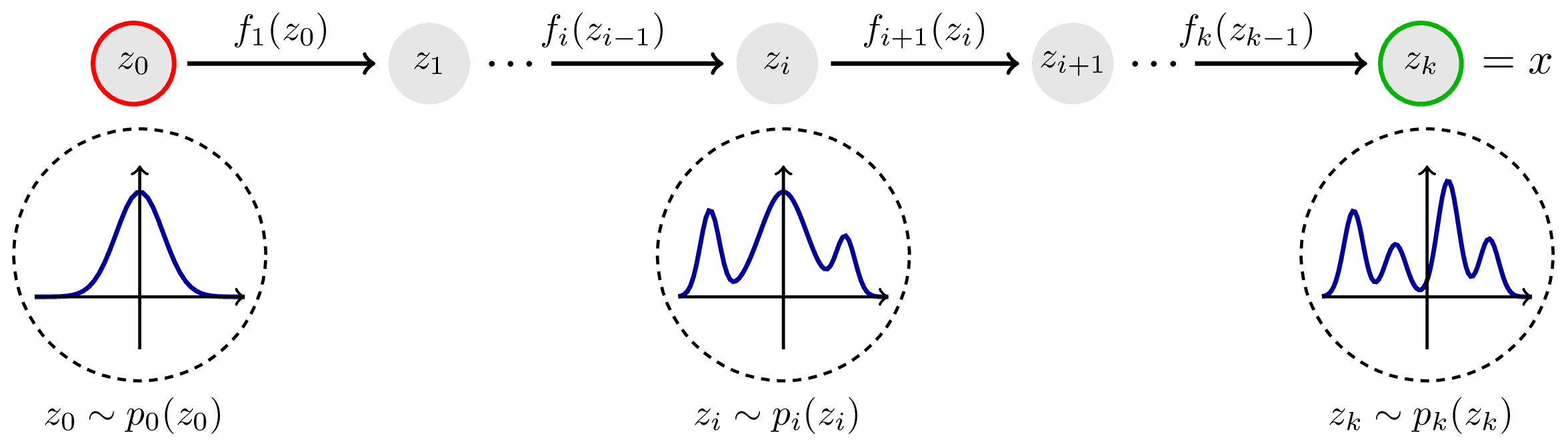
Image source: https://tikz.net/janosh/normalizing-flow.png
The key steps involved in the operation of normalizing flows are as follows (from left to right):
- Start with a simple, easy-to-sample distribution, usually a Gaussian, which serves as the "base" distribution
- Apply a series of invertible transformations to map the samples from the base distribution to the desired complex data distribution
- Each transformation in the flow must be reversible, meaning it has both a forward pass (sampling from the base distribution to the complex distribution) and an inverse pass (mapping samples from the complex distribution back to the base distribution)
- The flow ensures that the probability density function (PDF) of the complex distribution can be analytically calculated using the determinant of the Jacobian matrix resulting from the transformations
By stacking multiple transformations in a sequence, normalizing flows can model complex and multi-modal distributions while providing the ability to compute the likelihood of the data and perform efficient sampling in both directions (from base to complex and vice versa). However, it is important to note that since XGBoostLSS is based on a one vs. all estimation strategy, where a separate tree is grown for each parameter, estimating many parameters for a large dataset can become computationally expensive. For more details, we refer to our related paper Alexander März and Thomas Kneib (2022): Distributional Gradient Boosting Machines.
Imports
from xgboostlss.model import *
from xgboostlss.distributions.SplineFlow import *
from xgboostlss.distributions.flow_utils import NormalizingFlowClass
from xgboostlss.datasets.data_loader import load_simulated_gaussian_data
from scipy.stats import norm

import multiprocessing
import plotnine
from plotnine import *
plotnine.options.figure_size = (20, 10)
Data
# The data is simulated as a Gaussian, where x is the only true feature and all others are noise variables
    # loc = 10
    # scale = 1 + 4 * ((0.3 < x) & (x < 0.5)) + 2 * (x > 0.7)

train, test = load_simulated_gaussian_data()
n_cpu = multiprocessing.cpu_count()

X_train, y_train = train.filter(regex="x"), train["y"].values
X_test, y_test = test.filter(regex="x"), test["y"].values

dtrain = xgb.DMatrix(X_train, label=y_train, nthread=n_cpu)
dtest = xgb.DMatrix(X_test, nthread=n_cpu)
Select Normalizing Flow
In the following, we specify a list of candidate normalizing flows. The function flow_select returns the negative log-likelihood of each specification. The normalizing flow with the lowest negative log-likelihood is selected. The function also plots the density of the target variable and the fitted density, using the best suitable normalizing flow among the specified ones. However, note that choosing the best performing flow based solely on training data may lead to overfitting, since normalizing flows have a higher risk of overfitting compared to parametric distributions. When using normalizing flows, it is crucial to carefully select the specifications to strike a balance between model complexity and generalization ability.
# See ?SplineFlow for an overview.
bound = np.max([np.abs(y_train.min()), y_train.max()])
target_support = "real"

candidate_flows = [

    SplineFlow(target_support=target_support, count_bins=2,  bound=bound, order="linear"),
    SplineFlow(target_support=target_support, count_bins=4,  bound=bound, order="linear"),
    SplineFlow(target_support=target_support, count_bins=6,  bound=bound, order="linear"),
    SplineFlow(target_support=target_support, count_bins=8,  bound=bound, order="linear"),
    SplineFlow(target_support=target_support, count_bins=12, bound=bound, order="linear"),
    SplineFlow(target_support=target_support, count_bins=16, bound=bound, order="linear"),
    SplineFlow(target_support=target_support, count_bins=20, bound=bound, order="linear"),

    SplineFlow(target_support=target_support, count_bins=2,  bound=bound, order="quadratic"),
    SplineFlow(target_support=target_support, count_bins=4,  bound=bound, order="quadratic"),
    SplineFlow(target_support=target_support, count_bins=6,  bound=bound, order="quadratic"),
    SplineFlow(target_support=target_support, count_bins=8,  bound=bound, order="quadratic"),
    SplineFlow(target_support=target_support, count_bins=12, bound=bound, order="quadratic"),
    SplineFlow(target_support=target_support, count_bins=16, bound=bound, order="quadratic"),
    SplineFlow(target_support=target_support, count_bins=20, bound=bound, order="quadratic"),

]

flow_nll = NormalizingFlowClass().flow_select(target=y_train, candidate_flows=candidate_flows, max_iter=50, plot=True, figure_size=(12, 5))
flow_nll
Fitting of candidate normalizing flows completed: 100%|███████████████████████████████████████████████████████████████████████████████████████████████████████████████████████████████████████████████████████████████████████████████████████████████| 14/14 [00:51<00:00, 3.70s/it]

| nll | NormFlow | |
|---|---|---|
| rank | ||
| 1 | 16595.917006 | SplineFlow(count_bins: 20, order: linear) |
| 2 | 16608.693807 | SplineFlow(count_bins: 12, order: quadratic) |
| 3 | 16622.862265 | SplineFlow(count_bins: 16, order: quadratic) |
| 4 | 16640.156074 | SplineFlow(count_bins: 6, order: linear) |
| 5 | 16640.611035 | SplineFlow(count_bins: 16, order: linear) |
| 6 | 16649.404709 | SplineFlow(count_bins: 8, order: linear) |
| 7 | 16651.375456 | SplineFlow(count_bins: 8, order: quadratic) |
| 8 | 16653.378393 | SplineFlow(count_bins: 6, order: quadratic) |
| 9 | 16674.331780 | SplineFlow(count_bins: 12, order: linear) |
| 10 | 16822.629927 | SplineFlow(count_bins: 4, order: quadratic) |
| 11 | 16902.398862 | SplineFlow(count_bins: 20, order: quadratic) |
| 12 | 17538.588405 | SplineFlow(count_bins: 4, order: linear) |
| 13 | 17692.968508 | SplineFlow(count_bins: 2, order: linear) |
| 14 | 17737.569055 | SplineFlow(count_bins: 2, order: quadratic) |
Normalizing Flow Specification
Even though SplineFlow(count_bins: 20, order: linear) shows the best fit to the data, we choose a more parameter parsimonious specification (recall that a separate tree is grown for each parameter):
- for count_bins=20, we need to estimate 3*count_bins + (count_bins-1) = 79 parameters
- for count_bins=8, we need to estimate 3*count_bins + (count_bins-1) = 31 parameters
# Specifies Spline-Flow. See ?SplineFlow for an overview.
bound = np.max([np.abs(y_train.min()), y_train.max()])

xgblss = XGBoostLSS(
    SplineFlow(target_support="real",     # Specifies the support of the target. Options are "real", "positive", "positive_integer" or "unit_interval"
               count_bins=8,              # The number of segments comprising the spline.
               bound=bound,               # By adjusting the value, you can control the size of the bounding box and consequently control the range of inputs that the spline transform operates on.
               order="linear",            # The order of the spline. Options are "linear" or "quadratic".
               stabilization="None",      # Options are "None", "MAD" or "L2".
               loss_fn="nll"              # Loss function. Options are "nll" (negative log-likelihood) or "crps"(continuous ranked probability score).
            )
)
Hyper-Parameter Optimization
Any XGBoost hyperparameter can be tuned, where the structure of the parameter dictionary needs to be as follows:
- Float/Int sample_type
    - {"param_name": ["sample_type", low, high, log]}
        - sample_type: str, Type of sampling, e.g., "float" or "int"
        - low: int, Lower endpoint of the range of suggested values
        - high: int, Upper endpoint of the range of suggested values
        - log: bool, Flag to sample the value from the log domain or not
    - Example: {"eta": "float", low=1e-5, high=1, log=True]}

- Categorical sample_type
    - {"param_name": ["sample_type", ["choice1", "choice2", "choice3", "..."]]}
        - sample_type: str, Type of sampling, either "categorical"
        - choice1, choice2, choice3, ...: str, Possible choices for the parameter
    - Example: {"booster": ["categorical", ["gbtree", "dart"]]}

- For parameters without tunable choice (this is needed if tree_method = "gpu_hist" and gpu_id needs to be specified)
    - {"param_name": ["none", [value]]},
        - param_name: str, Name of the parameter
        - value: int, Value of the parameter
    - Example: {"gpu_id": ["none", [0]]}
Depending on which parameters are optimized, it might happen that some of them are not used, e.g., when {"booster": ["categorical", ["gbtree", "gblinear"]]} and {"max_depth": ["int", 1, 10, False]} are specified, max_depth is not used when gblinear is sampled, since it has no such argument.
param_dict = {
    "eta":              ["float", {"low": 1e-5,   "high": 1,     "log": True}],
    "max_depth":        ["int",   {"low": 1,      "high": 10,    "log": False}],
    "gamma":            ["float", {"low": 1e-8,   "high": 40,    "log": True}],
    "subsample":        ["float", {"low": 0.2,    "high": 1.0,   "log": False}],
    "colsample_bytree": ["float", {"low": 0.2,    "high": 1.0,   "log": False}],
    "min_child_weight": ["float", {"low": 1e-8,   "high": 500,   "log": True}],
    "booster":          ["categorical", ["gbtree"]]
}

np.random.seed(123)
opt_param = xgblss.hyper_opt(param_dict,
                             dtrain,
                             num_boost_round=100,        # Number of boosting iterations.
                             nfold=5,                    # Number of cv-folds.
                             early_stopping_rounds=20,   # Number of early-stopping rounds
                             max_minutes=1000,           # Time budget in minutes, i.e., stop study after the given number of minutes.
                             n_trials=100,               # The number of trials. If this argument is set to None, there is no limitation on the number of trials.
                             silence=False,              # Controls the verbosity of the trail, i.e., user can silence the outputs of the trail.
                             seed=123,                   # Seed used to generate cv-folds.
                             hp_seed=None                # Seed for random number generator used in the Bayesian hyperparameter search.
                            )
[I 2023-07-20 15:21:25,613] A new study created in memory with name: XGBoostLSS Hyper-Parameter Optimization
0%| | 0/100 [00:00<?, ?it/s]
[I 2023-07-20 15:22:30,946] Trial 0 finished with value: 6255.344043 and parameters: {'eta': 0.03692566115300059, 'max_depth': 4, 'gamma': 7.887574463976319e-08, 'subsample': 0.9144017805889704, 'colsample_bytree': 0.29974692606946474, 'min_child_weight': 2.1274056292372507e-07, 'booster': 'gbtree'}. Best is trial 0 with value: 6255.344043.
[I 2023-07-20 15:22:44,079] Trial 1 finished with value: 16614.029491999998 and parameters: {'eta': 0.0017154637091307261, 'max_depth': 7, 'gamma': 8.23346450464663e-07, 'subsample': 0.5893614292128422, 'colsample_bytree': 0.22046879379684717, 'min_child_weight': 1.0217730512063771e-06, 'booster': 'gbtree'}. Best is trial 0 with value: 6255.344043.
[I 2023-07-20 15:22:56,891] Trial 2 finished with value: 3504.441992 and parameters: {'eta': 2.7751871589547672e-05, 'max_depth': 6, 'gamma': 3.02777318294296e-07, 'subsample': 0.26524245101484456, 'colsample_bytree': 0.27746635000321973, 'min_child_weight': 6.426034557726815e-05, 'booster': 'gbtree'}. Best is trial 2 with value: 3504.441992.
[I 2023-07-20 15:24:03,745] Trial 3 finished with value: 3070.370508 and parameters: {'eta': 0.08292199572889684, 'max_depth': 5, 'gamma': 1.5182628894900233e-06, 'subsample': 0.9403786460943477, 'colsample_bytree': 0.34051787348973905, 'min_child_weight': 0.2522861634643369, 'booster': 'gbtree'}. Best is trial 3 with value: 3070.370508.
[I 2023-07-20 15:25:04,564] Trial 4 finished with value: 3330.1626466000002 and parameters: {'eta': 0.0001509832299785431, 'max_depth': 7, 'gamma': 2.756531681117656e-06, 'subsample': 0.45360605857266495, 'colsample_bytree': 0.7204182240441368, 'min_child_weight': 30.680516520620287, 'booster': 'gbtree'}. Best is trial 3 with value: 3070.370508.
[I 2023-07-20 15:25:18,187] Trial 5 finished with value: 379086.15 and parameters: {'eta': 0.830518425703511, 'max_depth': 3, 'gamma': 0.012299985715140278, 'subsample': 0.9711870084155301, 'colsample_bytree': 0.24611711490622082, 'min_child_weight': 0.0005629880692600968, 'booster': 'gbtree'}. Best is trial 3 with value: 3070.370508.
[I 2023-07-20 15:25:31,891] Trial 6 finished with value: 3498.6242188000006 and parameters: {'eta': 0.0003611895880336918, 'max_depth': 7, 'gamma': 0.03786187454142862, 'subsample': 0.5124745199562726, 'colsample_bytree': 0.3551315906394943, 'min_child_weight': 0.00940156145963303, 'booster': 'gbtree'}. Best is trial 3 with value: 3070.370508.
[I 2023-07-20 15:25:46,531] Trial 7 finished with value: 5983.7352538000005 and parameters: {'eta': 4.496946572176012e-05, 'max_depth': 7, 'gamma': 0.0047194293358602145, 'subsample': 0.9344902260740249, 'colsample_bytree': 0.948864562594103, 'min_child_weight': 0.0005306028753515352, 'booster': 'gbtree'}. Best is trial 3 with value: 3070.370508.
[I 2023-07-20 15:26:02,781] Trial 8 finished with value: 111347.4359374 and parameters: {'eta': 0.003469024418224711, 'max_depth': 9, 'gamma': 2.3721946640811852e-07, 'subsample': 0.971286805911628, 'colsample_bytree': 0.6956479802596798, 'min_child_weight': 1.745492550550714e-08, 'booster': 'gbtree'}. Best is trial 3 with value: 3070.370508.
[I 2023-07-20 15:26:17,780] Trial 9 finished with value: 3242.7606932 and parameters: {'eta': 0.24801010294899173, 'max_depth': 1, 'gamma': 0.607096851031229, 'subsample': 0.31815420752411927, 'colsample_bytree': 0.8599030202986522, 'min_child_weight': 0.03278105788018955, 'booster': 'gbtree'}. Best is trial 3 with value: 3070.370508.
[I 2023-07-20 15:26:30,849] Trial 10 finished with value: 3332.3609862 and parameters: {'eta': 0.032439573574320306, 'max_depth': 10, 'gamma': 6.856157934141567e-05, 'subsample': 0.753463330634383, 'colsample_bytree': 0.4473388149594849, 'min_child_weight': 264.48982201499797, 'booster': 'gbtree'}. Best is trial 3 with value: 3070.370508.
[I 2023-07-20 15:26:43,690] Trial 11 finished with value: 3259.6298828000004 and parameters: {'eta': 0.5844375923601339, 'max_depth': 1, 'gamma': 14.125852834419698, 'subsample': 0.24445640866266827, 'colsample_bytree': 0.5042856805135316, 'min_child_weight': 0.16785137409425205, 'booster': 'gbtree'}. Best is trial 3 with value: 3070.370508.
[I 2023-07-20 15:27:03,532] Trial 12 finished with value: 3222.1685058 and parameters: {'eta': 0.10743432797751593, 'max_depth': 1, 'gamma': 1.336930452029465e-08, 'subsample': 0.7794937123701792, 'colsample_bytree': 0.9870833686249794, 'min_child_weight': 0.535865544343811, 'booster': 'gbtree'}. Best is trial 3 with value: 3070.370508.
[I 2023-07-20 15:27:29,687] Trial 13 finished with value: 3039.6305176 and parameters: {'eta': 0.1313966761766938, 'max_depth': 3, 'gamma': 1.2885824737841825e-08, 'subsample': 0.7811960478381322, 'colsample_bytree': 0.9910806136654325, 'min_child_weight': 0.6798696113137718, 'booster': 'gbtree'}. Best is trial 13 with value: 3039.6305176.
[I 2023-07-20 15:28:34,025] Trial 14 finished with value: 3091.93291 and parameters: {'eta': 0.02486308401269763, 'max_depth': 4, 'gamma': 2.4223562057848944e-05, 'subsample': 0.7794301516088603, 'colsample_bytree': 0.596378998525593, 'min_child_weight': 4.149494288988884, 'booster': 'gbtree'}. Best is trial 13 with value: 3039.6305176.
[I 2023-07-20 15:29:26,465] Trial 15 finished with value: 3062.4055174 and parameters: {'eta': 0.12661561026668358, 'max_depth': 3, 'gamma': 1.2654967651703994e-08, 'subsample': 0.8592553385029919, 'colsample_bytree': 0.4007346733446969, 'min_child_weight': 0.5854364054560578, 'booster': 'gbtree'}. Best is trial 13 with value: 3039.6305176.
[I 2023-07-20 15:29:40,670] Trial 16 pruned. Trial was pruned at iteration 22.
[I 2023-07-20 15:29:53,687] Trial 17 finished with value: 3328.545508 and parameters: {'eta': 0.13980158809194015, 'max_depth': 3, 'gamma': 1.5215938995345315e-08, 'subsample': 0.8490492736409923, 'colsample_bytree': 0.45639549413029157, 'min_child_weight': 275.8648934425574, 'booster': 'gbtree'}. Best is trial 13 with value: 3039.6305176.
[I 2023-07-20 15:30:06,776] Trial 18 pruned. Trial was pruned at iteration 20.
[I 2023-07-20 15:30:24,686] Trial 19 finished with value: 3056.6981444 and parameters: {'eta': 0.6544509882244208, 'max_depth': 5, 'gamma': 0.00021163507207378848, 'subsample': 0.869732698237011, 'colsample_bytree': 0.900974180793565, 'min_child_weight': 2.7817029183422135, 'booster': 'gbtree'}. Best is trial 13 with value: 3039.6305176.
[I 2023-07-20 15:30:40,061] Trial 20 finished with value: 3058.3840821999997 and parameters: {'eta': 0.7634529963570388, 'max_depth': 5, 'gamma': 0.0003869011067576662, 'subsample': 0.8535815300763139, 'colsample_bytree': 0.9049612798090937, 'min_child_weight': 7.127603761119032, 'booster': 'gbtree'}. Best is trial 13 with value: 3039.6305176.
[I 2023-07-20 15:30:56,014] Trial 21 finished with value: 3044.4860838 and parameters: {'eta': 0.8750118182115282, 'max_depth': 5, 'gamma': 0.00025296042041120204, 'subsample': 0.8638909186170046, 'colsample_bytree': 0.9261561699617321, 'min_child_weight': 13.307993350012621, 'booster': 'gbtree'}. Best is trial 13 with value: 3039.6305176.
[I 2023-07-20 15:31:11,403] Trial 22 finished with value: 3041.409082 and parameters: {'eta': 0.8678687545966929, 'max_depth': 6, 'gamma': 0.0003034358805344321, 'subsample': 0.9994750305856172, 'colsample_bytree': 0.9364531239253467, 'min_child_weight': 56.353446165160015, 'booster': 'gbtree'}. Best is trial 13 with value: 3039.6305176.
[I 2023-07-20 15:31:28,256] Trial 23 finished with value: 3045.8405272 and parameters: {'eta': 0.3091862911564756, 'max_depth': 6, 'gamma': 0.0008102771849499481, 'subsample': 0.992327967436072, 'colsample_bytree': 0.9538912185657742, 'min_child_weight': 56.324078030880365, 'booster': 'gbtree'}. Best is trial 13 with value: 3039.6305176.
[I 2023-07-20 15:31:40,479] Trial 24 finished with value: 3337.1875489999998 and parameters: {'eta': 0.2648285825517022, 'max_depth': 8, 'gamma': 4.72524211489433e-06, 'subsample': 0.8070969086041984, 'colsample_bytree': 0.9883810337379536, 'min_child_weight': 422.58538326701074, 'booster': 'gbtree'}. Best is trial 13 with value: 3039.6305176.
[I 2023-07-20 15:32:23,836] Trial 25 finished with value: 3049.2964354 and parameters: {'eta': 0.06430418453639147, 'max_depth': 4, 'gamma': 4.88444011961088e-05, 'subsample': 0.999397426898831, 'colsample_bytree': 0.8029295391032494, 'min_child_weight': 38.633122585967484, 'booster': 'gbtree'}. Best is trial 13 with value: 3039.6305176.
[I 2023-07-20 15:32:38,187] Trial 26 finished with value: 3054.6845702 and parameters: {'eta': 0.8614115024975222, 'max_depth': 6, 'gamma': 8.28703977696704e-06, 'subsample': 0.9044185260330364, 'colsample_bytree': 0.8032378041387337, 'min_child_weight': 22.700459833842594, 'booster': 'gbtree'}. Best is trial 13 with value: 3039.6305176.
[I 2023-07-20 15:33:01,784] Trial 27 finished with value: 3068.4505369999997 and parameters: {'eta': 0.29355992688035293, 'max_depth': 2, 'gamma': 0.00014032641956213097, 'subsample': 0.8180607845945178, 'colsample_bytree': 0.9958248821107969, 'min_child_weight': 0.056030271157428396, 'booster': 'gbtree'}. Best is trial 13 with value: 3039.6305176.
[I 2023-07-20 15:33:16,971] Trial 28 finished with value: 3042.01167 and parameters: {'eta': 0.9489949657070117, 'max_depth': 4, 'gamma': 0.0011531286846959436, 'subsample': 0.8974919764569149, 'colsample_bytree': 0.9200095124201007, 'min_child_weight': 1.2080542972828012, 'booster': 'gbtree'}. Best is trial 13 with value: 3039.6305176.
[I 2023-07-20 15:33:32,518] Trial 29 pruned. Trial was pruned at iteration 21.
[I 2023-07-20 15:33:46,149] Trial 30 pruned. Trial was pruned at iteration 21.
[I 2023-07-20 15:33:59,322] Trial 31 finished with value: 3043.5458494 and parameters: {'eta': 0.9957731824745992, 'max_depth': 5, 'gamma': 0.0012004496934510645, 'subsample': 0.8822741327587181, 'colsample_bytree': 0.9453127201123616, 'min_child_weight': 10.535252278624212, 'booster': 'gbtree'}. Best is trial 13 with value: 3039.6305176.
[I 2023-07-20 15:34:16,372] Trial 32 finished with value: 3037.6239746 and parameters: {'eta': 0.3759370865943818, 'max_depth': 4, 'gamma': 0.002280606215198254, 'subsample': 0.9310445013233254, 'colsample_bytree': 0.9993191393162827, 'min_child_weight': 1.351438052883453, 'booster': 'gbtree'}. Best is trial 32 with value: 3037.6239746.
[I 2023-07-20 15:34:33,533] Trial 33 finished with value: 3040.1080566 and parameters: {'eta': 0.38934599890918614, 'max_depth': 4, 'gamma': 8.296441273857323e-07, 'subsample': 0.9515796871722452, 'colsample_bytree': 0.9997532130387258, 'min_child_weight': 0.43235469432563967, 'booster': 'gbtree'}. Best is trial 32 with value: 3037.6239746.
[I 2023-07-20 15:34:55,933] Trial 34 finished with value: 3039.5586914 and parameters: {'eta': 0.18115338358393857, 'max_depth': 4, 'gamma': 6.166305075098885e-07, 'subsample': 0.945716328699108, 'colsample_bytree': 0.9865423390725786, 'min_child_weight': 0.19544651220436385, 'booster': 'gbtree'}. Best is trial 32 with value: 3037.6239746.
[I 2023-07-20 15:35:48,666] Trial 35 finished with value: 3038.745459 and parameters: {'eta': 0.04745485570053381, 'max_depth': 4, 'gamma': 5.975889221470206e-07, 'subsample': 0.9302528610335031, 'colsample_bytree': 0.9977485806465173, 'min_child_weight': 0.3298767479525565, 'booster': 'gbtree'}. Best is trial 32 with value: 3037.6239746.
[I 2023-07-20 15:36:03,076] Trial 36 pruned. Trial was pruned at iteration 20.
[I 2023-07-20 15:36:38,232] Trial 37 finished with value: 3072.348535 and parameters: {'eta': 0.1676023650818225, 'max_depth': 2, 'gamma': 1.3456281350922575e-06, 'subsample': 0.7312226777053694, 'colsample_bytree': 0.96403972726024, 'min_child_weight': 0.15659509459600862, 'booster': 'gbtree'}. Best is trial 32 with value: 3037.6239746.
[I 2023-07-20 15:36:51,718] Trial 38 pruned. Trial was pruned at iteration 20.
[I 2023-07-20 15:37:04,904] Trial 39 pruned. Trial was pruned at iteration 20.
[I 2023-07-20 15:37:35,193] Trial 40 finished with value: 3044.7080080000005 and parameters: {'eta': 0.16675746943436404, 'max_depth': 5, 'gamma': 4.394096661445257e-07, 'subsample': 0.9523079200049536, 'colsample_bytree': 0.7652455247039238, 'min_child_weight': 0.16742962289315963, 'booster': 'gbtree'}. Best is trial 32 with value: 3037.6239746.
[I 2023-07-20 15:37:53,559] Trial 41 finished with value: 3042.2968752 and parameters: {'eta': 0.4462381749855381, 'max_depth': 4, 'gamma': 1.7146100810737851e-06, 'subsample': 0.9622380196093626, 'colsample_bytree': 0.9974175750245168, 'min_child_weight': 0.383713251217408, 'booster': 'gbtree'}. Best is trial 32 with value: 3037.6239746.
[I 2023-07-20 15:38:11,673] Trial 42 finished with value: 3044.6321288 and parameters: {'eta': 0.3778012420288047, 'max_depth': 3, 'gamma': 4.663173144169329e-07, 'subsample': 0.923687326741991, 'colsample_bytree': 0.9979073897811195, 'min_child_weight': 2.2641120684946663, 'booster': 'gbtree'}. Best is trial 32 with value: 3037.6239746.
[I 2023-07-20 15:38:36,702] Trial 43 finished with value: 3036.498877 and parameters: {'eta': 0.17388192674987513, 'max_depth': 4, 'gamma': 6.309051431253172e-08, 'subsample': 0.9566651333215987, 'colsample_bytree': 0.9607007825565661, 'min_child_weight': 0.7675989664161897, 'booster': 'gbtree'}. Best is trial 43 with value: 3036.498877.
[I 2023-07-20 15:39:12,740] Trial 44 finished with value: 3040.2740722 and parameters: {'eta': 0.09206794072353378, 'max_depth': 4, 'gamma': 5.6489289726626155e-08, 'subsample': 0.8954928691334318, 'colsample_bytree': 0.8784043381395148, 'min_child_weight': 1.1433654917851803, 'booster': 'gbtree'}. Best is trial 43 with value: 3036.498877.
[I 2023-07-20 15:39:26,547] Trial 45 pruned. Trial was pruned at iteration 21.
[I 2023-07-20 15:39:58,144] Trial 46 finished with value: 3036.6901368000003 and parameters: {'eta': 0.1120307552445573, 'max_depth': 5, 'gamma': 3.7580746615978925e-08, 'subsample': 0.9789698093894728, 'colsample_bytree': 0.9644330946571384, 'min_child_weight': 0.2561065047964661, 'booster': 'gbtree'}. Best is trial 43 with value: 3036.498877.
[I 2023-07-20 15:40:12,361] Trial 47 finished with value: 317827.7375 and parameters: {'eta': 0.043706750220849286, 'max_depth': 6, 'gamma': 3.913006896332813e-08, 'subsample': 0.9690969467883341, 'colsample_bytree': 0.9072431124346024, 'min_child_weight': 0.001461751094675627, 'booster': 'gbtree'}. Best is trial 43 with value: 3036.498877.
[I 2023-07-20 15:40:25,665] Trial 48 pruned. Trial was pruned at iteration 20.
[I 2023-07-20 15:40:48,546] Trial 49 finished with value: 3042.2581054 and parameters: {'eta': 0.1931007050198132, 'max_depth': 7, 'gamma': 7.094687769779725e-07, 'subsample': 0.9992028340293483, 'colsample_bytree': 0.8590260387503983, 'min_child_weight': 0.21836876632154886, 'booster': 'gbtree'}. Best is trial 43 with value: 3036.498877.
[I 2023-07-20 15:41:04,123] Trial 50 pruned. Trial was pruned at iteration 20.
[I 2023-07-20 15:41:33,545] Trial 51 finished with value: 3037.9859862000003 and parameters: {'eta': 0.11608170004318419, 'max_depth': 3, 'gamma': 1.1356448351699668e-08, 'subsample': 0.9616677986985251, 'colsample_bytree': 0.964418076021131, 'min_child_weight': 0.31618597066744286, 'booster': 'gbtree'}. Best is trial 43 with value: 3036.498877.
[I 2023-07-20 15:42:09,265] Trial 52 finished with value: 3037.8550293999997 and parameters: {'eta': 0.11507600724744876, 'max_depth': 4, 'gamma': 2.199638902174226e-08, 'subsample': 0.9695617768158347, 'colsample_bytree': 0.9121099339048496, 'min_child_weight': 0.07206419964863138, 'booster': 'gbtree'}. Best is trial 43 with value: 3036.498877.
[I 2023-07-20 15:42:45,858] Trial 53 finished with value: 3042.282959 and parameters: {'eta': 0.09578923298517399, 'max_depth': 3, 'gamma': 2.3214886659640414e-08, 'subsample': 0.9704644240551171, 'colsample_bytree': 0.8861859676783096, 'min_child_weight': 0.08976940730880904, 'booster': 'gbtree'}. Best is trial 43 with value: 3036.498877.
[I 2023-07-20 15:43:02,356] Trial 54 finished with value: 3046.4572264 and parameters: {'eta': 0.4863009899191616, 'max_depth': 5, 'gamma': 2.933694891028008e-08, 'subsample': 0.9219233858526725, 'colsample_bytree': 0.918018970862546, 'min_child_weight': 0.57477971522028, 'booster': 'gbtree'}. Best is trial 43 with value: 3036.498877.
[I 2023-07-20 15:43:15,596] Trial 55 pruned. Trial was pruned at iteration 20.
[I 2023-07-20 15:43:29,306] Trial 56 pruned. Trial was pruned at iteration 20.
[I 2023-07-20 15:43:46,722] Trial 57 finished with value: 3046.938037 and parameters: {'eta': 0.48143764278934603, 'max_depth': 10, 'gamma': 3.306952790316785e-08, 'subsample': 0.8797070161002929, 'colsample_bytree': 0.9688852153874727, 'min_child_weight': 5.035373364625581, 'booster': 'gbtree'}. Best is trial 43 with value: 3036.498877.
[I 2023-07-20 15:44:07,802] Trial 58 finished with value: 3040.500879 and parameters: {'eta': 0.23122542961969572, 'max_depth': 5, 'gamma': 1.074776154118335e-08, 'subsample': 0.9791431780517371, 'colsample_bytree': 0.8373987685965062, 'min_child_weight': 1.3021503329254518, 'booster': 'gbtree'}. Best is trial 43 with value: 3036.498877.
[I 2023-07-20 15:44:44,348] Trial 59 finished with value: 3038.3109863999994 and parameters: {'eta': 0.12288738314201289, 'max_depth': 6, 'gamma': 1.0261606944828545e-07, 'subsample': 0.9313884266044806, 'colsample_bytree': 0.8747675594194785, 'min_child_weight': 0.4314497637179585, 'booster': 'gbtree'}. Best is trial 43 with value: 3036.498877.
[I 2023-07-20 15:45:16,683] Trial 60 finished with value: 3034.6042479999996 and parameters: {'eta': 0.131715522890815, 'max_depth': 8, 'gamma': 8.595351520871723e-08, 'subsample': 0.8467450878672628, 'colsample_bytree': 0.8921093053178858, 'min_child_weight': 5.529194250117682, 'booster': 'gbtree'}. Best is trial 60 with value: 3034.6042479999996.
[I 2023-07-20 15:45:55,507] Trial 61 finished with value: 3033.7231936 and parameters: {'eta': 0.12878869661672784, 'max_depth': 9, 'gamma': 1.1134506962884295e-07, 'subsample': 0.979008136534911, 'colsample_bytree': 0.8774303224098216, 'min_child_weight': 2.6230072911913602, 'booster': 'gbtree'}. Best is trial 61 with value: 3033.7231936.
[I 2023-07-20 15:46:16,992] Trial 62 finished with value: 3034.4493164 and parameters: {'eta': 0.23951274541935214, 'max_depth': 9, 'gamma': 2.4451144212121893e-08, 'subsample': 0.9989539360739352, 'colsample_bytree': 0.8999224216276656, 'min_child_weight': 7.489966946988934, 'booster': 'gbtree'}. Best is trial 61 with value: 3033.7231936.
[I 2023-07-20 15:46:36,107] Trial 63 finished with value: 3034.496631 and parameters: {'eta': 0.2906285342066211, 'max_depth': 9, 'gamma': 2.3320028783573044e-07, 'subsample': 0.998545496085736, 'colsample_bytree': 0.900876478262415, 'min_child_weight': 11.882340482031697, 'booster': 'gbtree'}. Best is trial 61 with value: 3033.7231936.
[I 2023-07-20 15:46:56,817] Trial 64 finished with value: 3035.3720216 and parameters: {'eta': 0.2820047348161208, 'max_depth': 9, 'gamma': 2.184155692311592e-07, 'subsample': 0.996343223272909, 'colsample_bytree': 0.8381661712662352, 'min_child_weight': 18.587468085803913, 'booster': 'gbtree'}. Best is trial 61 with value: 3033.7231936.
[I 2023-07-20 15:47:12,480] Trial 65 finished with value: 3047.7063965999996 and parameters: {'eta': 0.5798351672744028, 'max_depth': 9, 'gamma': 2.378427771818312e-07, 'subsample': 0.994049449129419, 'colsample_bytree': 0.8375069604498476, 'min_child_weight': 19.32650734634661, 'booster': 'gbtree'}. Best is trial 61 with value: 3033.7231936.
[I 2023-07-20 15:47:35,243] Trial 66 finished with value: 3034.7572264 and parameters: {'eta': 0.2498196015404798, 'max_depth': 9, 'gamma': 9.388235442649892e-08, 'subsample': 0.9892227950699081, 'colsample_bytree': 0.7821132557310545, 'min_child_weight': 5.695495978260237, 'booster': 'gbtree'}. Best is trial 61 with value: 3033.7231936.
[I 2023-07-20 15:47:47,709] Trial 67 pruned. Trial was pruned at iteration 20.
[I 2023-07-20 15:48:07,900] Trial 68 finished with value: 3034.8570802 and parameters: {'eta': 0.2405533104908695, 'max_depth': 9, 'gamma': 7.837410655297795e-08, 'subsample': 0.9015583204840619, 'colsample_bytree': 0.8511509480054339, 'min_child_weight': 7.834999223021249, 'booster': 'gbtree'}. Best is trial 61 with value: 3033.7231936.
[I 2023-07-20 15:48:28,141] Trial 69 finished with value: 3040.0000976 and parameters: {'eta': 0.2956399924280415, 'max_depth': 8, 'gamma': 9.88751541731488e-08, 'subsample': 0.9022556763576, 'colsample_bytree': 0.7719874184705332, 'min_child_weight': 8.25004890534742, 'booster': 'gbtree'}. Best is trial 61 with value: 3033.7231936.
[I 2023-07-20 15:48:43,765] Trial 70 pruned. Trial was pruned at iteration 24.
[I 2023-07-20 15:49:07,476] Trial 71 finished with value: 3032.0960452 and parameters: {'eta': 0.2265464552295039, 'max_depth': 9, 'gamma': 6.650095266635949e-08, 'subsample': 0.9538124529289038, 'colsample_bytree': 0.8659924086826483, 'min_child_weight': 5.605164868653055, 'booster': 'gbtree'}. Best is trial 71 with value: 3032.0960452.
[I 2023-07-20 15:49:27,374] Trial 72 finished with value: 3038.8958494000003 and parameters: {'eta': 0.22902007353151901, 'max_depth': 10, 'gamma': 1.1515183939981256e-07, 'subsample': 0.901785004503644, 'colsample_bytree': 0.8588347755027981, 'min_child_weight': 30.385739895404505, 'booster': 'gbtree'}. Best is trial 71 with value: 3032.0960452.
[I 2023-07-20 15:49:45,395] Trial 73 finished with value: 3044.8246092 and parameters: {'eta': 0.35260837690076746, 'max_depth': 9, 'gamma': 1.1106991827582779e-06, 'subsample': 0.9398513983516278, 'colsample_bytree': 0.8895583767246401, 'min_child_weight': 5.98719906547585, 'booster': 'gbtree'}. Best is trial 71 with value: 3032.0960452.
[I 2023-07-20 15:49:58,678] Trial 74 pruned. Trial was pruned at iteration 20.
[I 2023-07-20 15:50:14,877] Trial 75 finished with value: 3043.1111816 and parameters: {'eta': 0.6183195923598164, 'max_depth': 10, 'gamma': 2.732262054750231e-07, 'subsample': 0.8822019431362266, 'colsample_bytree': 0.8220732908570513, 'min_child_weight': 11.748022411721493, 'booster': 'gbtree'}. Best is trial 71 with value: 3032.0960452.
[I 2023-07-20 15:50:40,403] Trial 76 finished with value: 3037.9492189999996 and parameters: {'eta': 0.23855793927016783, 'max_depth': 9, 'gamma': 3.992529445417728e-08, 'subsample': 0.951313051091195, 'colsample_bytree': 0.8950261415738519, 'min_child_weight': 3.476577441804782, 'booster': 'gbtree'}. Best is trial 71 with value: 3032.0960452.
[I 2023-07-20 15:50:53,113] Trial 77 pruned. Trial was pruned at iteration 20.
[I 2023-07-20 15:51:05,514] Trial 78 pruned. Trial was pruned at iteration 20.
[I 2023-07-20 15:51:24,012] Trial 79 finished with value: 3040.228418 and parameters: {'eta': 0.33335306038090784, 'max_depth': 9, 'gamma': 3.4761652743022766e-07, 'subsample': 0.9453491076334737, 'colsample_bytree': 0.7488837947306157, 'min_child_weight': 31.895005763179608, 'booster': 'gbtree'}. Best is trial 71 with value: 3032.0960452.
[I 2023-07-20 15:51:57,058] Trial 80 finished with value: 3031.0040528 and parameters: {'eta': 0.14277821773718294, 'max_depth': 10, 'gamma': 8.088782592976787e-07, 'subsample': 0.9977974732766702, 'colsample_bytree': 0.809525144421714, 'min_child_weight': 7.514977546259929, 'booster': 'gbtree'}. Best is trial 80 with value: 3031.0040528.
[I 2023-07-20 15:52:34,886] Trial 81 finished with value: 3036.6441894 and parameters: {'eta': 0.14688542814891956, 'max_depth': 10, 'gamma': 7.038891673481538e-08, 'subsample': 0.9928503505941781, 'colsample_bytree': 0.8085460732808113, 'min_child_weight': 7.665893011318919, 'booster': 'gbtree'}. Best is trial 80 with value: 3031.0040528.
[I 2023-07-20 15:52:51,975] Trial 82 finished with value: 3050.27583 and parameters: {'eta': 0.4379462106578011, 'max_depth': 9, 'gamma': 6.000344883817363e-07, 'subsample': 0.9971102122143154, 'colsample_bytree': 0.8273389607051485, 'min_child_weight': 23.10361905636443, 'booster': 'gbtree'}. Best is trial 80 with value: 3031.0040528.
[I 2023-07-20 15:53:19,354] Trial 83 finished with value: 3036.3837402 and parameters: {'eta': 0.22417761641274248, 'max_depth': 10, 'gamma': 1.2867623022100379e-06, 'subsample': 0.9577715079481326, 'colsample_bytree': 0.8747482876335879, 'min_child_weight': 3.382772126945124, 'booster': 'gbtree'}. Best is trial 80 with value: 3031.0040528.
[I 2023-07-20 15:53:59,165] Trial 84 finished with value: 3031.5499022 and parameters: {'eta': 0.07777175813083295, 'max_depth': 9, 'gamma': 1.7185510203212536e-07, 'subsample': 0.9348510407500364, 'colsample_bytree': 0.9329988917156696, 'min_child_weight': 13.528526200805464, 'booster': 'gbtree'}. Best is trial 80 with value: 3031.0040528.
[I 2023-07-20 15:54:12,033] Trial 85 pruned. Trial was pruned at iteration 20.
[I 2023-07-20 15:54:37,014] Trial 86 finished with value: 3031.0340822 and parameters: {'eta': 0.16516782634436789, 'max_depth': 10, 'gamma': 1.7234931690405196e-08, 'subsample': 0.9342372920085978, 'colsample_bytree': 0.909095200137177, 'min_child_weight': 9.871149485232598, 'booster': 'gbtree'}. Best is trial 80 with value: 3031.0040528.
[I 2023-07-20 15:55:07,366] Trial 87 finished with value: 3036.349414 and parameters: {'eta': 0.13339295383590416, 'max_depth': 10, 'gamma': 2.3445324150229605e-08, 'subsample': 0.9325053962950647, 'colsample_bytree': 0.9360339455632799, 'min_child_weight': 2.085188759176219, 'booster': 'gbtree'}. Best is trial 80 with value: 3031.0040528.
[I 2023-07-20 15:55:32,779] Trial 88 finished with value: 3034.3476564 and parameters: {'eta': 0.17185470709215206, 'max_depth': 10, 'gamma': 1.5232308495682677e-08, 'subsample': 0.9554709654420762, 'colsample_bytree': 0.9012439729356523, 'min_child_weight': 13.647558912144003, 'booster': 'gbtree'}. Best is trial 80 with value: 3031.0040528.
[I 2023-07-20 15:55:46,546] Trial 89 pruned. Trial was pruned at iteration 20.
[I 2023-07-20 15:55:59,914] Trial 90 pruned. Trial was pruned at iteration 20.
[I 2023-07-20 15:56:29,402] Trial 91 finished with value: 3037.1376950000003 and parameters: {'eta': 0.1801027949508445, 'max_depth': 9, 'gamma': 1.4836461200734805e-07, 'subsample': 0.977567003551009, 'colsample_bytree': 0.8711392022063783, 'min_child_weight': 4.944097482180133, 'booster': 'gbtree'}. Best is trial 80 with value: 3031.0040528.
[I 2023-07-20 15:56:53,676] Trial 92 finished with value: 3043.7844238000002 and parameters: {'eta': 0.1464197811613084, 'max_depth': 10, 'gamma': 1.969266532609399e-08, 'subsample': 0.9768054797862559, 'colsample_bytree': 0.8959052698638602, 'min_child_weight': 38.86530610694329, 'booster': 'gbtree'}. Best is trial 80 with value: 3031.0040528.
[I 2023-07-20 15:57:14,050] Trial 93 finished with value: 3045.8321287999997 and parameters: {'eta': 0.35648020407239445, 'max_depth': 9, 'gamma': 5.1544279890441144e-08, 'subsample': 0.9410417761633629, 'colsample_bytree': 0.9321853495782388, 'min_child_weight': 1.9636483287430881, 'booster': 'gbtree'}. Best is trial 80 with value: 3031.0040528.
[I 2023-07-20 15:57:40,873] Trial 94 finished with value: 3037.1115236 and parameters: {'eta': 0.19774996151749544, 'max_depth': 8, 'gamma': 3.7637323222116544e-07, 'subsample': 0.9599639239639111, 'colsample_bytree': 0.8708399930343282, 'min_child_weight': 4.99726808337303, 'booster': 'gbtree'}. Best is trial 80 with value: 3031.0040528.
[I 2023-07-20 15:57:55,309] Trial 95 pruned. Trial was pruned at iteration 20.
[I 2023-07-20 15:58:30,377] Trial 96 finished with value: 3037.8553222 and parameters: {'eta': 0.12748413134085249, 'max_depth': 9, 'gamma': 1.5262247871791894e-07, 'subsample': 0.9791566175763764, 'colsample_bytree': 0.8853711291798442, 'min_child_weight': 21.67053566526402, 'booster': 'gbtree'}. Best is trial 80 with value: 3031.0040528.
[I 2023-07-20 15:58:49,951] Trial 97 finished with value: 3043.8745604000005 and parameters: {'eta': 0.4864981430946289, 'max_depth': 7, 'gamma': 7.539816084962301e-08, 'subsample': 0.8933603644872811, 'colsample_bytree': 0.922160705746178, 'min_child_weight': 2.6831925998799897, 'booster': 'gbtree'}. Best is trial 80 with value: 3031.0040528.
[I 2023-07-20 15:59:05,830] Trial 98 pruned. Trial was pruned at iteration 21.
[I 2023-07-20 15:59:40,344] Trial 99 finished with value: 3040.4043948 and parameters: {'eta': 0.1875688877271209, 'max_depth': 9, 'gamma': 1.0222902239978172e-07, 'subsample': 0.9427128387025056, 'colsample_bytree': 0.8100148150348059, 'min_child_weight': 0.8118029486547931, 'booster': 'gbtree'}. Best is trial 80 with value: 3031.0040528.

Hyper-Parameter Optimization successfully finished.
  Number of finished trials:  100
  Best trial:
    Value: 3031.0040528
    Params:
    eta: 0.14277821773718294
    max_depth: 10
    gamma: 8.088782592976787e-07
    subsample: 0.9977974732766702
    colsample_bytree: 0.809525144421714
    min_child_weight: 7.514977546259929
    booster: gbtree
    opt_rounds: 30
Model Training
np.random.seed(123)

opt_params = opt_param.copy()
n_rounds = opt_params["opt_rounds"]
del opt_params["opt_rounds"]

# Train Model with optimized hyperparameters
xgblss.train(opt_params,
             dtrain,
             num_boost_round=n_rounds
             )
Prediction
# Set seed for reproducibility
torch.manual_seed(123)

# Number of samples to draw from predicted distribution
n_samples = 10000
# Quantiles to calculate from predicted distribution
quant_sel = [0.05, 0.95]

# Sample from predicted distribution
pred_samples = xgblss.predict(dtest,
                              pred_type="samples",
                              n_samples=n_samples,
                              seed=123)

# Calculate quantiles from predicted distribution
pred_quantiles = xgblss.predict(dtest,
                                pred_type="quantiles",
                                n_samples=n_samples,
                                quantiles=quant_sel)

# Returns predicted parameters
pred_params = xgblss.predict(dtest,
                             pred_type="parameters")
pred_samples.head()
| y_sample0 | y_sample1 | y_sample2 | y_sample3 | y_sample4 | y_sample5 | y_sample6 | y_sample7 | y_sample8 | y_sample9 | ... | y_sample9990 | y_sample9991 | y_sample9992 | y_sample9993 | y_sample9994 | y_sample9995 | y_sample9996 | y_sample9997 | y_sample9998 | y_sample9999 | |
|---|---|---|---|---|---|---|---|---|---|---|---|---|---|---|---|---|---|---|---|---|---|
| 0 | 12.476486 | 11.232409 | 4.531297 | 11.363811 | 4.781734 | 13.938910 | 11.681598 | 14.658313 | 9.974003 | 8.736984 | ... | 13.760765 | 9.338540 | 8.213298 | 11.582684 | 9.699373 | 15.296181 | 5.445426 | 10.907387 | 11.825034 | 6.373481 |
| 1 | 16.861736 | 8.414603 | 10.939034 | 13.475651 | 8.340402 | 10.276856 | 12.489843 | 10.608356 | 12.365025 | 9.093086 | ... | 10.898591 | 2.581861 | 11.356403 | 13.315522 | 6.913608 | 15.685884 | 9.282003 | 9.755927 | 3.866492 | 10.277873 |
| 2 | 12.442025 | 9.501931 | 9.579384 | 11.448649 | 15.371767 | 11.944936 | 11.200554 | 9.318138 | 9.043898 | 10.726871 | ... | 10.183985 | 11.545186 | 8.312314 | 10.584079 | 8.789487 | 10.342226 | 9.892250 | 8.029637 | 10.462024 | 10.342827 |
| 3 | 11.241399 | 8.752618 | 13.266323 | 3.948052 | 16.326685 | 16.667992 | 8.063462 | 17.408077 | 6.992835 | 10.044690 | ... | -0.004205 | 8.638702 | 17.228178 | 7.539776 | 3.437411 | 8.712561 | 13.743514 | 13.827578 | 13.600298 | 8.999898 |
| 4 | 13.759394 | 8.122649 | 6.028914 | 4.139555 | 5.615580 | 10.576174 | 6.294752 | 15.667155 | 10.416535 | 16.968143 | ... | 9.751814 | 7.578747 | 8.704581 | 12.697542 | 8.643000 | 7.352739 | 14.508101 | 10.728389 | 7.371967 | 9.274317 |
5 rows × 10000 columns
pred_quantiles.head()
| quant_0.05 | quant_0.95 | |
|---|---|---|
| 0 | 5.147843 | 15.415341 |
| 1 | 5.348317 | 15.360555 |
| 2 | 7.733128 | 12.995715 |
| 3 | 0.741641 | 18.253794 |
| 4 | 3.127059 | 16.718515 |
pred_params.head()
| param_1 | param_2 | param_3 | param_4 | param_5 | param_6 | param_7 | param_8 | param_9 | param_10 | ... | param_22 | param_23 | param_24 | param_25 | param_26 | param_27 | param_28 | param_29 | param_30 | param_31 | |
|---|---|---|---|---|---|---|---|---|---|---|---|---|---|---|---|---|---|---|---|---|---|
| 0 | -0.280689 | -0.156779 | -0.461753 | -0.831503 | 0.182882 | -0.557738 | -2.383831 | 1.173182 | 0.97675 | 0.290846 | ... | 0.511808 | 0.286395 | 0.945506 | 0.805746 | 0.692724 | 0.634053 | -0.886691 | 4.017344 | 0.745495 | 1.069772 |
| 1 | -0.280689 | -0.156779 | -0.461753 | -0.831503 | 0.182882 | -0.557738 | -2.383831 | 1.173182 | 0.97675 | 0.290846 | ... | 0.480639 | 0.286395 | 0.945506 | 0.805746 | 0.692724 | 0.634053 | -0.977325 | 3.833302 | 0.745495 | 1.069772 |
| 2 | -0.280689 | -0.156779 | -0.461753 | -0.831503 | 0.182882 | -0.557738 | -2.383831 | 1.173182 | 0.97675 | 0.290846 | ... | 0.359091 | 0.286395 | 0.945506 | 0.805746 | 0.692724 | 0.634053 | -2.301708 | 3.418404 | 0.745495 | 1.069772 |
| 3 | -0.280689 | -0.156779 | -0.461753 | -0.831503 | 0.182882 | -0.557738 | -2.383831 | 1.173182 | 0.97675 | 0.290846 | ... | 0.315179 | 0.286395 | 0.945506 | 0.805746 | 0.692724 | 0.634053 | 0.802579 | 1.476677 | 0.745495 | 1.069772 |
| 4 | -0.280689 | -0.156779 | -0.461753 | -0.831503 | 0.182882 | -0.557738 | -2.383831 | 1.173182 | 0.97675 | 0.290846 | ... | 0.210731 | 0.286395 | 0.945506 | 0.805746 | 0.692724 | 0.634053 | 0.025325 | 3.645396 | 0.745495 | 1.069772 |
5 rows × 31 columns
SHAP Interpretability
Note that in contrast to parametric distributions, the parameters of the Spline-Flow do not have a direct interpretation.
# Partial Dependence Plot of how x acts on param_21
xgblss.plot(X_test,
            parameter="param_21",
            feature="x_true",
            plot_type="Partial_Dependence")


# Feature Importance of param_21
xgblss.plot(X_test,
            parameter="param_21",
            plot_type="Feature_Importance")

Plot of Actual vs. Predicted Quantiles
np.random.seed(123)

###
# Actual Quantiles
###
q1 = norm.ppf(quant_sel[0], loc = 10, scale = 1 + 4*((0.3 < test["x_true"].values) & (test["x_true"].values < 0.5)) + 2*(test["x_true"].values > 0.7))
q2 = norm.ppf(quant_sel[1], loc = 10, scale = 1 + 4*((0.3 < test["x_true"].values) & (test["x_true"].values < 0.5)) + 2*(test["x_true"].values > 0.7))
test["quant"] = np.where(test["y"].values < q1, 0, np.where(test["y"].values < q2, 1, 2))
test["alpha"] = np.where(test["y"].values <= q1, 1, np.where(test["y"].values >= q2, 1, 0))
df_quantiles = test[test["alpha"] == 1]

# Lower Bound
yl = list(set(q1))
yl.sort()
yl = [yl[2],yl[0],yl[2],yl[1],yl[1]]
sfunl = pd.DataFrame({"x_true":[0, 0.3, 0.5, 0.7, 1], "y":yl})

# Upper Bound
yu = list(set(q2))
yu.sort()
yu = [yu[0],yu[2],yu[0],yu[1],yu[1]]
sfunu = pd.DataFrame({"x_true":[0, 0.3, 0.5, 0.7, 1], "y":yu})

###
# Predicted Quantiles
###
test["lb"] = pred_quantiles.iloc[:,0]
test["ub"] = pred_quantiles.iloc[:,1]

###
# Plot
###
(ggplot(test,
        aes("x_true",
            "y")) +
 geom_point(alpha = 0.2, color = "black", size = 2) +
 theme_bw(base_size=15) +
 theme(legend_position="none",
       plot_title = element_text(hjust = 0.5)) +
 labs(title = "XGBoostLSS Regression - Simulated Data Example",
      x="x")  +
 geom_line(aes("x_true",
               "ub"),
           size = 1,
           color = "blue",
           alpha = 0.7) +
 geom_line(aes("x_true",
               "lb"),
           size = 1,
           color = "blue",
           alpha = 0.7) +
 geom_point(df_quantiles,
            aes("x_true",
                "y"),
            color = "red",
            alpha = 0.7,
            size = 2) +
 geom_step(sfunl,
           aes("x_true",
               "y"),
           size = 1,
           linetype = "dashed")  +
 geom_step(sfunu,
           aes("x_true",
               "y"),
           size = 1,
           linetype = "dashed")
)

<Figure Size: (2000 x 1000)>
True vs. Predicted Distributional Parameters
In the following figure, we compare the true parameters of the Gaussian with the ones predicted by XGBoostLSS. The below figure shows that the estimated parameters closely match the true ones (recall that the location parameter $\mu=10$ is simulated as being a constant).
dist_params = ["loc", "scale"]

# Calculate parameters from samples
sample_params = pd.DataFrame.from_dict(
    {
        "loc": pred_samples.mean(axis=1),
        "scale": pred_samples.std(axis=1),
        "x_true": X_test["x_true"].values
    }
)

# Data with predicted values
plot_df_predt = pd.melt(sample_params[["x_true"] + dist_params],
                        id_vars="x_true",
                        value_vars=dist_params)
plot_df_predt["type"] = "PREDICT"

# Data with actual values
plot_df_actual = pd.melt(test[["x_true"] + dist_params],
                         id_vars="x_true",
                         value_vars=dist_params)
plot_df_actual["type"] = "TRUE"

# Combine data for plotting
plot_df = pd.concat([plot_df_predt, plot_df_actual])
plot_df["variable"] = plot_df.variable.str.upper()
plot_df["type"] = pd.Categorical(plot_df["type"], categories = ["PREDICT", "TRUE"])

# Plot
(ggplot(plot_df,
        aes(x="x_true",
            y="value",
            color="type")) +
 geom_line(size=1.1) +
 facet_wrap("variable",
            scales="free") +
 labs(title="Parameters of univariate Gaussian predicted with XGBoostLSS",
      x="",
      y="") +
 theme_bw(base_size=15) +
 theme(legend_position="bottom",
       plot_title = element_text(hjust = 0.5),
       legend_title = element_blank())
)

<Figure Size: (2000 x 1000)>
Density Plots
pred_df = pd.melt(pred_samples.iloc[:,0:5])
actual_df = pd.DataFrame.from_dict({"variable": "ACTUAL", "value": y_test.reshape(-1,)})
plot_df = pd.concat([pred_df, actual_df])

(
    ggplot(plot_df,
           aes(x="value",
               color="variable",
               fill="variable")) +
    geom_density(alpha=0.4) +
    facet_wrap("variable",
               ncol=2) +
    theme_bw(base_size=15) +
    theme(plot_title = element_text(hjust = 0.5)) +
    theme(legend_position="none")
)

<Figure Size: (2000 x 1000)>
Actual vs. Predicted
Since we predict the entire conditional distribution, we can overlay the point predictions with predicted densities, from which we can also derive quantiles of interest.
y_pred = []

n_examples = 8
q_sel = [0.05, 0.95]
y_sel=0
samples_arr = pred_samples.values.reshape(-1,n_samples)

for i in range(n_examples):
    y_samples = pd.DataFrame(samples_arr[i,:].reshape(-1,1), columns=["PREDICT_DENSITY"])
    y_samples["PREDICT_POINT"] = y_samples["PREDICT_DENSITY"].mean()
    y_samples["PREDICT_Q05"] = y_samples["PREDICT_DENSITY"].quantile(q=q_sel[0])
    y_samples["PREDICT_Q95"] = y_samples["PREDICT_DENSITY"].quantile(q=q_sel[1])
    y_samples["ACTUAL"] = y_test[i]
    y_samples["obs"]= f"Obervation {i+1}"
    y_pred.append(y_samples)

pred_df = pd.melt(pd.concat(y_pred, axis=0), id_vars="obs")
pred_df["obs"] = pd.Categorical(pred_df["obs"], categories=[f"Obervation {i+1}" for i in range(n_examples)])
df_actual, df_pred_dens, df_pred_point, df_q05, df_q95 = [x for _, x in pred_df.groupby("variable")]

plot_pred = (
    ggplot(pred_df,
           aes(color="variable")) +
    stat_density(df_pred_dens,
                 aes(x="value"),
                 size=1.1) +
    geom_point(df_pred_point,
               aes(x="value",
                   y=0),
               size=1.4) +
    geom_point(df_actual,
               aes(x="value",
                   y=0),
               size=1.4) +
    geom_vline(df_q05,
               aes(xintercept="value",
                   fill="variable",
                   color="variable"),
               linetype="dashed",
               size=1.1) +
    geom_vline(df_q95,
               aes(xintercept="value",
                   fill="variable",
                   color="variable"),
               linetype="dashed",
               size=1.1) +
    facet_wrap("obs",
               scales="free",
               ncol=4) +
    labs(title="Predicted vs. Actual \n",
         x = "") +
    theme_bw(base_size=15) +
    theme(plot_title = element_text(hjust = 0.5)) +
    scale_fill_brewer(type="qual", palette="Dark2") +
    theme(legend_position="bottom",
          legend_title = element_blank()
         )
)

print(plot_pred)
